Download
1 / 28
280 likes | 292 Views
Chapter 8: Major Elements. “Wet-chems”: gravimetric/volumetric. Chapter 8: Major Elements. Modern Spectroscopic Techniques. Figure 8.1. The geometry of typical spectroscopic instruments. From Winter (2001) An Introduction to Igneous and Metamorphic Petrology. Prentice Hall. Element.

E N D
Chapter 8: Major Elements “Wet-chems”: gravimetric/volumetric
Chapter 8: Major Elements Modern Spectroscopic Techniques Figure 8.1.The geometry of typical spectroscopic instruments. From Winter (2001) An Introduction to Igneous and Metamorphic Petrology. Prentice Hall.
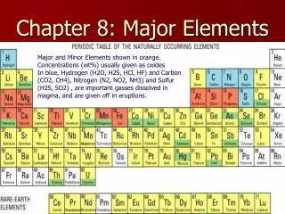
Element Wt % Oxide Atom % O 60.8 Si 59.3 21.2 Al 15.3 6.4 Fe 7.5 2.2 Ca 6.9 2.6 Mg 4.5 2.4 Na 2.8 1.9 Abundance of the elements in the Earth’s crust Major elements: usually greater than 1% SiO2 Al2O3 FeO* MgO CaO Na2O K2O H2O Minor elements: usually 0.1 - 1% TiO2 MnO P2O5 CO2 Trace elements: usually < 0.1% everything else
Wt. % Oxides to Atom % Conversion Oxide Wt. % Mol Wt. Atom prop Atom % SiO 49.20 60.09 0.82 12.25 2 TiO 1.84 95.90 0.02 0.29 2 Al O 15.74 101.96 0.31 4.62 2 3 Fe O 3.79 159.70 0.05 0.71 2 3 FeO 7.13 71.85 0.10 1.48 MnO 0.20 70.94 0.00 0.04 MgO 6.73 40.31 0.17 2.50 CaO 9.47 56.08 0.17 2.53 Na O 2.91 61.98 0.09 1.40 2 K O 1.10 94.20 0.02 0.35 2 + H O 0.95 18.02 0.11 1.58 2 (O) 4.83 72.26 Total 99.06 6.69 100.00 A typical rock analysis Must multiply by # of cations in oxide
Table 8-3. Chemical analyses of some representative igneous rocks Peridotite Basalt Andesite Rhyolite Phonolite SiO2 42.26 49.20 57.94 72.82 56.19 TiO2 0.63 1.84 0.87 0.28 0.62 Al2O3 4.23 15.74 17.02 13.27 19.04 Fe2O3 3.61 3.79 3.27 1.48 2.79 FeO 6.58 7.13 4.04 1.11 2.03 MnO 0.41 0.20 0.14 0.06 0.17 MgO 31.24 6.73 3.33 0.39 1.07 CaO 5.05 9.47 6.79 1.14 2.72 Na2O 0.49 2.91 3.48 3.55 7.79 K2O 0.34 1.10 1.62 4.30 5.24 H2O+ 3.91 0.95 0.83 1.10 1.57 Total 98.75 99.06 99.3 99.50 99.23
CIPW Norm • Mode is the volume % of minerals seen • Normis a calculated “idealized” mineralogy
Variation Diagrams How do we display chemical data in a meaningful way?
Bivariate (x-y) diagrams Harker diagram for Crater Lake Figure 8.2.Harker variation diagram for 310 analyzed volcanic rocks from Crater Lake (Mt. Mazama), Oregon Cascades. Data compiled by Rick Conrey (personal communication).
Bivariate (x-y) diagrams Harker diagram for Crater Lake Figure 8.2.Harker variation diagram for 310 analyzed volcanic rocks from Crater Lake (Mt. Mazama), Oregon Cascades. Data compiled by Rick Conrey (personal communication).
Ternary Variation Diagrams Example: AFM diagram (alkalis-FeO*-MgO) Figure 8.2.AFM diagram for Crater Lake volcanics, Oregon Cascades. Data compiled by Rick Conrey (personal communication).
Table 8-5 . Chemical analyses (wt. %) of a hypothetical set of related volcanics. Oxide B BA A D RD R SiO 50.2 54.3 60.1 64.9 66.2 71.5 2 TiO 1.1 0.8 0.7 0.6 0.5 0.3 2 Al O 14.9 15.7 16.1 16.4 15.3 14.1 2 3 Fe O * 10.4 9.2 6.9 5.1 5.1 2.8 2 3 MgO 7.4 3.7 2.8 1.7 0.9 0.5 CaO 10.0 8.2 5.9 3.6 3.5 1.1 Na O 2.6 3.2 3.8 3.6 3.9 3.4 2 K O 1.0 2.1 2.5 2.5 3.1 4.1 2 LOI 1.9 2.0 1.8 1.6 1.2 1.4 Total 99.5 99.2 100.6 100.0 99.7 99.2 B = basalt, BA = basaltic andesite, A = andesite, D = dacite, RD = rhyo-dacite, R = rhyolite. Data from Ragland (1989) Models of Magmatic Evolution
Figure 8.7.Stacked variation diagrams of hypothetical components X and Y (either weight or mol %). P = parent, D = daughter, S = solid extract, A, B, C = possible extracted solid phases. For explanation, see text. From Ragland (1989). Basic Analytical Petrology, Oxford Univ. Press.
Harker diagram • Smooth trends • Model with 3 assumptions: 1 Rocks are related by FX 2 Trends = liquid line of descent 3 The basalt is the parent magma from which the others are derived Figure 8.7.Stacked variation diagrams of hypothetical components X and Y (either weight or mol %). P = parent, D = daughter, S = solid extract, A, B, C = possible extracted solid phases. For explanation, see text. From Ragland (1989). Basic Analytical Petrology, Oxford Univ. Press.
Extrapolate BA B and further to low SiO2 • K2O is first element to 0 (at SiO2 = 46.5) • 46.5% SiO2 is interpreted to be the concentration in the bulk solid extract and the blue line the concentration of all other oxides Figure 8.7.Stacked variation diagrams of hypothetical components X and Y (either weight or mol %). P = parent, D = daughter, S = solid extract, A, B, C = possible extracted solid phases. For explanation, see text. From Ragland (1989). Basic Analytical Petrology, Oxford Univ. Press.
Extrapolate the other curves back BA B blue line and read off X of mineral extract Results: Remove plagioclase, olivine, pyroxene and Fe-Ti oxide Oxide Wt% Cation Norm SiO2 46.5 ab 18.3 TiO2 1.4 an 30.1 Al2O3 14.2 di 23.2 Fe2O3* 11.5 hy 4.7 MgO 10.8 ol 19.3 CaO 11.5 mt 1.7 Na2O 2.1 il 2.7 K2O 0 Total 98.1 100 Then repeat for each increment BA A etc.
Figure 8.8. Variation diagram on a cation basis for the fractional crystallization of olivine, augite, and plagioclase to form BA from B (Table 8-6). From Ragland (1989). Basic Analytical Petrology, Oxford Univ. Press.
Figure 8.9. Equilateral triangle showing the solution to the bulk mineral extract (shaded area) best fitting the criteria for the variation diagrams in Figure 8-8. From Ragland (1989). Basic Analytical Petrology, Oxford Univ. Press.
Magma Series Can chemistry be used to distinguish families of magma types?
Early on it was recognized that some chemical parameters were very useful in regard to distinguishing magmatic groups • Total Alkalis (Na2O + K2O) • Silica (SiO2) and silica saturation • Alumina (Al2O3)
Alkali vs. Silica diagram for Hawaiian volcanics: Seems to be two distinct groupings: alkaline and subalkaline Figure 8.11. Total alkalis vs. silica diagram for the alkaline and sub-alkaline rocks of Hawaii. After MacDonald (1968). GSA Memoir 116
The Basalt Tetrahedron and the Ne-Ol-Q base Alkaline and subalkaline fields are again distinct Figure 8.12.Left: the basalt tetrahedron (after Yoder and Tilley, 1962). J. Pet., 3, 342-532. Right: the base of the basalt tetrahedron using cation normative minerals, with the compositions of subalkaline rocks (black) and alkaline rocks (gray) from Figure 8-11, projected from Cpx. After Irvine and Baragar (1971). Can. J. Earth Sci., 8, 523-548.
1713 Liquid Thermal Divide Tr + L Ne + L Ab + L Ab + L 1070 1060 Ne + Ab Ab + Tr Q Ne Ab Thermal divide separates the silica-saturated (subalkaline) from the silica-undersaturated (alkaline) fields at low pressure Cannot cross this divide by FX, so can’t derive one series from the other (at least via low-P FX)
F o l h e T i i t i c Calc-alkaline M A AFM diagram: can further subdivide the subalkaline magma series into a tholeiitic and a calc-alkaline series Figure 8.14.AFM diagram showing the distinction between selected tholeiitic rocks from Iceland, the Mid-Atlantic Ridge, the Columbia River Basalts, and Hawaii (solid circles) plus the calc-alkaline rocks of the Cascade volcanics (open circles). From Irving and Baragar (1971). After Irvine and Baragar (1971). Can. J. Earth Sci., 8, 523-548.
Figure 18.2.Alumina saturation classes based on the molar proportions of Al2O3/(CaO+Na2O+K2O) (“A/CNK”) after Shand (1927). Common non-quartzo-feldspathic minerals for each type are included. After Clarke (1992). Granitoid Rocks. Chapman Hall.
Figure 8-10 a.Plot of CaO (green) and (Na2O + K2O) (red) vs. SiO2 for the Crater Lake data. Peacock (1931) used the value of SiO2 at which the two curves crossed as his “alkali-lime index” (dashed line). b. Alumina saturation indices (Shand, 1927) with analyses of the peraluminous granitic rocks from the Achala Batholith, Argentina (Lira and Kirschbaum, 1990).In S. M. Kay and C. W. Rapela (eds.), Plutonism from Antarctica to Alaska. Geol. Soc. Amer. Special Paper, 241. pp. 67-76.
A world-wide survey suggests that there may be some important differences between the three series After Wilson (1989). Igneous Petrogenesis. Unwin Hyman - Kluwer