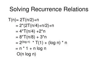
Download
1 / 34
350 likes | 367 Views
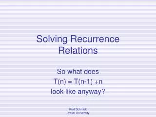
Solving recurrence equations. 5 techniques for solving recurrence equations: Recursion tree Iteration method Induction (Guess and Test) Master Theorem (master method) Characteristic equations We concentrate on the recursion tree method (others in the book).

E N D
Solving recurrence equations • 5 techniques for solving recurrence equations: • Recursion tree • Iteration method • Induction (Guess and Test) • Master Theorem (master method) • Characteristic equations • We concentrate on the recursion tree method (others in the book) cutler: divide & conquer
Deriving the count using the recursion tree method • Recursion trees provide a convenient way to represent the unrolling of recursive algorithm • It is not a formal proof but a good technique to compute the count. • Once the tree is generated, each node contains its “non recursive number of operations” t(n) or DirectSolutionCount • The count is derived by summing the “non recursive number of operations” of all the nodes in the tree • For convenience we usually compute the sum for all nodes at each given depth, and then sum these sums over all depths. cutler: divide & conquer
Building the recursion tree • The initial recursion tree has a single node containing two fields: • The recursive call, (for example Factorial(n)) and • the corresponding count T(n) . • The tree is generated by: • unrolling the recursion of the node depth 0, • then unrolling the recursion for the nodes at depth 1, etc. • The recursion is unrolled as long as the size of the recursive call is greater than DirectSolutionSize cutler: divide & conquer
Building the recursion tree • When the “recursion is unrolled”, each current leaf node is substituted by a subtree containing a root and a child for each recursive call done by the algorithm. • The root of the subtree contains the recursive call, and the corresponding “non recursive count”. • Each child node contains a recursive call, and its corresponding count. • The unrolling continues, until the “size” in the recursive call is DirectSolutionSize • Nodes with a call of DirectSolutionSize, are not “unrolled”, and their count is replaced by DirectSolutionCount cutler: divide & conquer
Factorial(n) T(n) Example: recursive factorial • Initially, the recursive tree is a node containing the call to Factorial(n), and count T(n). • When we unroll the computation this node is replaced with a subtree containing a root and one child: • The root of the subtree contains the call to Factorial(n) , and the “non recursive count” for this call t(n)= (1). • The child node contains the recursive call to Factorial(n-1), and the count for this call, T(n-1). cutler: divide & conquer
Factorial(n) Factorial(n-1) t(n)= (1) T(n-1) After the first unrolling depth ndT(n) 0 1 (1) 1 1 T(n-1) nd denotes the number of nodes at that depth cutler: divide & conquer
Factorial(n) Factorial(n-1) Factorial(n-2) t(n)= (1) t(n-1)= (1) T(n-2) After the second unrolling depth ndT(n) 0 1 (1) 1 1 (1) 2 1 T(n-2) cutler: divide & conquer
Factorial(n) Factorial(n-1) Factorial(n-2) Factorial(n-3) t(n)= (1) t(n-1)= (1) t(n-2)= (1) T(n-3) After the third unrolling depth ndT(n) 0 1 (1) 1 1 (1) 2 1 (1) 3 1 T(n-3) For FactorialDirectSolutionSize =1and DirectSolutionCount= (1) cutler: divide & conquer
Factorial(n-1) Factorial(n-3) Factorial(n-2) Factorial(1) Factorial(n) t(n)= (1) t(n-1)= (1) T(1)= t(n-3)= (1) t(n-2)= (1) The recursion tree depth ndT(n) 0 1 (1) 1 1 (1) 2 1 (1) 3 1 (1) (1) n-1 1 T(1)= (1) The sum T(n)=n* (1) = (n) cutler: divide & conquer
Divide and Conquer • Basic idea: divide a problem into smaller portions, solve the smaller portions and combine the results. • Name some algorithms you already know that employ this technique. • D&C is a top down approach. Often, you use recursion to implement D&C algorithms. • The following is an “outline” of a divide and conquer algorithm cutler: divide & conquer
Divide and Conquer procedure Solution(I); begin if size(I) <=smallSize then {calculate solution} return(DirectSolution(I)) {use direct solution} else {decompose, solve each and combine} Decompose(I, I1,...,Ik); for i:=1 to k do S(i):=Solution(Ii); {solve a smaller problem} end {for} return(Combine(S1,...,Sk)); {combine solutions} end {Solution} cutler: divide & conquer
Divide and Conquer • Let size(I) = n • DirectSolutionCount = DS(n) • t(n) = D(n) + C(n) where: • D(n) = count for dividing problem into subproblems • C(n) = count for combining solutions cutler: divide & conquer
Divide and Conquer • Main advantages • Simple code • Often efficient algorithms • Suitable for parallel computation cutler: divide & conquer
Binary search • Assumption - the list S[low…high] is sorted, and x is the search key • If the search key x is in the list, x==S[i], and the index i is returned. • If x is not in the list a NoSuchKey is returned • Book’s version: returns an index i where x would be inserted into the sorted list cutler: divide & conquer
Binary search • The problem is divided into 3 subproblems: x=S[mid], xÎ S[low,..,mid-1], xÎ S[mid+1,..,high] • The first case x=S[mid]) is easily solved • The other cases xÎ S[low,..,mid-1], or xÎ S[mid+1,..,high] require a recursive call • When the array is empty the search terminates with a “non-index value” cutler: divide & conquer
BinarySearch(S, k, low, high) if low > high then return NoSuchKey else mid floor ((low+high)/2) if (k == S[mid]) returnmid else if (k < S[mid]) then return BinarySearch(S, k, low, mid-1) else return BinarySearch(S, k, mid+1, high) cutler: divide & conquer
Worst case analysis • A worst input (what is it?) causes the algorithm to keep searching until low>high • We count number of comparisons of a list element with x per recursive call. • Assume 2k n < 2k+1k = ëlg nû • T (n) - worst case number of comparisons for the call to BS(n) cutler: divide & conquer
BS(n) T(n) Recursion tree for BinarySearch (BS) • Initially, the recursive tree is a node containing the call to BS(n), and total amount of work in the worst case, T(n). • When we unroll the computation this node is replaced with a subtree containing a root and one child: • The root of the subtree contains the call to BS(n) , and the “nonrecursive work” for this call t(n). • The child node contains the recursive call to BS(n/2), and the total amount of work in the worst case for this call, T(n/2). cutler: divide & conquer
BS(n) BS(n/2) t(n)=1 T(n/2) After first unrolling depth ndT(n) 0 1 1 1 1 T(n/2) cutler: divide & conquer
BS(n) BS(n/2) BS(n/4) t(n)=1 t(n/2)=1 T(n/4) After second unrolling depth ndT(n) 0 1 1 1 1 1 2 1 T(n/4) cutler: divide & conquer
BS(n) BS(n/2) BS(n/4) BS(n/8) t(n)=1 t(n/2)=1 t(n/4)=1 T(n/8) After third unrolling depth ndT(n) 0 1 1 1 1 1 1 1 1 T(n/8) For BinarySearchDirectSolutionSize =0,1and DirectSolutionCount=0 for 0, and 1 for 1 cutler: divide & conquer
Terminating the unrolling • Let 2kn < 2k+1 • k= lg n • When a node has a call to BS(n/2k), (or to BS(n/2k+1)): • The size of the list is DirectSolutionSize since n/2k =1, (or n/2k+1 =0) • In this case the unrolling terminates, and the node is a leaf containing DirectSolutionCount (DFC) = 1, (or 0) cutler: divide & conquer
BS(n) BS(n/2) BS(n/4) BS(n/2k) t(n)=1 t(n/2)=1 t(n/4)=1 DFC=1 The recursion tree depth ndT(n) 0 1 1 1 1 1 2 1 1 k 1 1 T(n)=k+1=lgn +1 cutler: divide & conquer
Merge Sort Input: S of size n. Output: a permutation of S, such that if i > j then S[ i ] S[ j ] Divide: If S has at least 2 elements divide into S1 and S2. S1 contains the the first n/2 elements of S.S2 has the last n/2 elements of S. Recurs: Recursively sort S1 , and S2. Conquer: Merge sorted S1 and S2 into S. cutler: divide & conquer
Merge Sort: Input: S1 if (n 2) 2 moveFirst(S, S1, (n+1)/2))// divide3 moveSecond(S, S2, n/2) // divide4 Sort(S1) // recurs5 Sort(S2) // recurs6 Merge( S1, S2, S) // conquer cutler: divide & conquer
Merge( S1 , S2, S ): Pseudocode Input: S1 , S2, sorted in nondecreasing order OutputS is a sorted sequence.1. while (S1 is Not Empty && S2 is Not Empty)2. if (S1.first() S2.first() )3. remove first element of S1 and move it to the end ofS4. else remove first element of S2 and move it to the end ofS5. move the remaining elements of the non-empty sequence (S1 or S2 )to S cutler: divide & conquer
Recurrence Equation for MergeSort. • The implementation of the moves costsQ(n) and the merge costs Q(n). So the total count for dividing and merging is Q(n). • The recurrence relation for the run time of MergeSort is T(n) = T( n/2) + T( n/2) + Q(n) . T(1) = Q(1) cutler: divide & conquer
MS(n) T(n) Recursion tree for MergeSort (MS) • Initially, the recursive tree is a node containing the call to MS(n), and total amount of work in the worst case, T(n). • When we unroll the computation this node is replaced with a subtree: • The root of the subtree contains the call to MS(n) , and the “nonrecursive work” for this call t(n). • The two children contain a recursive call to MS(n/2), and the total amount of work in the worst case for this call, T(n/2). cutler: divide & conquer
MS(n/2) MS(n/2) T(n/2) T(n/2) After first unrolling of mergeSort MS(n) depth ndT(n) t(n)=(n) 0 1 (n) 2T(n/2) cutler: divide & conquer
MS(n/2) MS(n/4) MS(n/4) MS(n/4) MS(n/4) (n/2) T(n/4) T(n/4) T(n/4) T(n/4) MS(n) MS(n/2) (n/2) (n) After second unrolling depth ndT(n) 0 1 (n) 1 2 (n) + 4T(n/4) cutler: divide & conquer
MS(n/2) MS(n/8) MS(n/8) MS(n/8) MS(n/4) MS(n/4) MS(n/4) MS(n/4) (n/2) (n/4) (n/4) (n/4) (n/4) T(n/8) T(n/8) T(n/8) MS(n/2) MS(n) (n) (n/2) After third unrolling depth ndT(n) 0 1 (n) 1 2 (n) + 2 4 (n) + + + 8T(n/8) cutler: divide & conquer
Terminating the unrolling • For simplicity let n = 2k • lg n = k • When a node has a call to MS(n/2k): • The size of the list to merge sort is DirectSolutionSize since n/2k =1 • In this case the unrolling terminates, and the node is a leaf containing DirectSolutionCount = (1) cutler: divide & conquer
Q(n/20) Q(n/ 21) Q(n/ 21) Q(n/ 22) Q(n/ 22) Q(n / 22) Q(n/ 22) Q(n/ 23) Q(n/ 8) Q(n/ 8) Q(n/ 8) Q(n/ 8) Q(n/ 8) Q(n/ 8) Q(n/ 8) Q(1) Q(1) The recursion tree (excluding the calls) d nd T(n) 0 1 Q(n) 1 2 Q(n) 2 4 Q(n) 3 8 Q(n) k 2k Q(n) T(n)= (k+1)Q(n)= Q( n lg n) cutler: divide & conquer
d=0 nd=1: Q(n ) d=1 nd=2: 21 ´ Q n æ ö 22 ´ Q d=2 nd=22: = Q (n) ç ÷ è ø 21 . . . n æ ö = Q (n) d=knd=2k: ç ÷ ø è 22 The sum for each depth cutler: divide & conquer