Download
1 / 34
340 likes | 489 Views
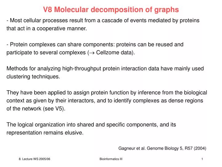
V8 Molecular decomposition of graphs. - Most cellular processes result from a cascade of events mediated by proteins that act in a cooperative manner. Protein complexes can share components: proteins can be reused and participate to several complexes ( Cellzome data).

E N D
V8 Molecular decomposition of graphs • - Most cellular processes result from a cascade of events mediated by proteins that act in a cooperative manner. • Protein complexes can share components: proteins can be reused and participate to several complexes ( Cellzome data). • Methods for analyzing high-throughput protein interaction data have mainly used clustering techniques. • They have been applied to assign protein function by inference from the biological context as given by their interactors, and to identify complexes as dense regions of the network (see V5). • The logical organization into shared and specific components, and its representation remains elusive. Gagneur et al. Genome Biology 5, R57 (2004) Bioinformatics III
shared components Shared components = proteins or groups of proteins occurring in different complexes are fairly common: A shared component may be a small part of many complexes, acting as a unit that is constantly reused for ist function. Also, it may be the main part of the complex e.g. in a family of variant complexes that differ from each other by distinct proteins that provide functional specificity. Aim: identify and properly represent the modularity of protein-protein interaction networks by identifying the shared components and the way they are arranged to generate complexes. Gagneur et al. Genome Biology 5, R57 (2004) Georg Casari, Cellzome (Heidelberg) Bioinformatics III
Modules A graph and its modules. Nodes connected by a link are called neighbors. In graph theory, a module is a set of nodes that have the same neighbors outside the module. In addition to the trivial modules{a},{b},...,{g} and {a,b,c,..,g}, this graph contains the modules {a,b,c}, {a,b},{a,c},{b,c} and {e,f}. Gagneur et al. Genome Biology 5, R57 (2004) Bioinformatics III
Quotient • Elements of a module have exactly the same neighbors outside the module • one can substitute all of them for a representative node. In a quotient, all elements of the module are replaced by the representative node, and the edges with the neighbors are replaced by edges to the representative. Quotients can be iterated until the entire graph is merged into a final representative node. Iterated quotients can be captured in a tree, where each node represents a module, which is a subset of its parent and the set of its descendant leaves. Gagneur et al. Genome Biology 5, R57 (2004) Bioinformatics III
Modular decomposition Modular decomposition of the example graph shown before. Modular decomposition gives a labeled tree that represents iterations of particular quotients, here the successive quotients on the modules {a,b,c} and {e,f}. The modular decomposition is a unique, canonical tree of iterated quotients (formal proof exists Möhring 1985, V9). Gagneur et al. Genome Biology 5, R57 (2004) Bioinformatics III
Nodes The nodes of the modular decomposition are categorized in 3 ways: series : the direct descendants are all neighbors of each other, (labelled by an asterisk within a circle) parallel : the direct descendants are all non-neighbors of each other, (labelled by two parallel lines within a circle) prime : by the structure of the module otherwise (prime module case). (labelled by a P within a circle) The graph can be retrieved from the tree on the right by recursively expanding the modules using the information in the labels. Therefore, the labeled tree can be seen as an exact alternative representation of the graph. Gagneur et al. Genome Biology 5, R57 (2004) Bioinformatics III
Results from protein complex purifications (PCP), e.g. TAP • Different types of data: • Y2H: detects direct physical interactions between proteins • PCP by tandem affinity purification with mass-spectrometric identification of the protein components identifies multi-protein complexes • Molecular decomposition will have a different meaning due to different semantics of such graphs. Here, focus analysis on PCP content. PCP experiment: select bait protein where TAP-label is attached Co-purify protein with those proteins that co-occur in at least one complex with the bait protein. Gagneur et al. Genome Biology 5, R57 (2004) Bioinformatics III
Clique and maximal clique A clique is a fully connected sub-graph, that is, a set of nodes that are all neighbors of each other. In this example, the whole graph is a clique and consequently any subset of it is also a clique, for example {a,c,d,e} or {b,e}. A maximal clique is a clique that is not contained in any larger clique. Here only {a,b,c,d,e} is a maximal clique. Assuming complete datasets and ideal results, a permanent complex will appear as a clique. The opposite is not true: not every clique in the network necessarily derives from an existing complex. E.g. 3 connected proteins can be the outcome of a single trimer, 3 heterodimers or combinations thereof. Gagneur et al. Genome Biology 5, R57 (2004) Bioinformatics III
Results from protein complex purifications (PCP), e.g. TAP Interpretation of graph and module labels for systematic PCP experiments. (a) Two neighbors in the network are proteins occurring in a same complex. (b) Several potential sets of complexes can be the origin of the same observed network. Restricting interpretation to the simplest model (top right), the series module reads as a logical AND between its members. (c) A module labeled ´parallel´ corresponds to proteins or modules working as strict alternatives with respect to their common neighbors. (d) The ´prime´ case is a structure where none of the two previous cases occurs. Gagneur et al. Genome Biology 5, R57 (2004) Bioinformatics III
Obtain maximal cliques Modular decomposition provides an instruction set to deliver all maximal cliques of a graph. In particular, when the decomposition has only series and parallels, the maximal cliques are straightforwardly retrieved by traversing the tree recursively from top to bottom. A series module acts as a product: the maximal cliques are all the combinations made up of one maximal clique from each „child“ node. A parallel module acts as a sum: the set of maximal cliques is the union of all maximal cliques from the „child“ nodes. Gagneur et al. Genome Biology 5, R57 (2004) Bioinformatics III
Interpretation for PCP protein interaction networks In the modular decomposition tree, the leaves are proteins, the root represents the whole network. In between, each node is a module that is a sub-part of ist parent. The label of a node gives the nature of the relationship between ist direct children. Proteins or modules in a parallel module can be be seen as alternatives. If A is neighbor of B and C, which are not neighbors of each other, then A can belong to a complex together with either B or C, but not with both at the same time. B and C define a parallel module and thus are alternative partners in a complex with their common neighbor A. This situation corresponds to a logical „exclusive OR“ between B and C. Gagneur et al. Genome Biology 5, R57 (2004) Bioinformatics III
Interpretation for PCP protein interaction networks Proteins or modules in a series module can be seen as potentially combined in any way. If A is neighbor of B and C, and B and C are also neighbors, the A can belong to a complex together with B or C, or with both at the same time. This corresponds to a logical „OR“ between B and C. A series module can be seen as a unit: a set of proteins (modules) that function together. A ‚prime‘ is a graph where neither of these cases occurs. Gagneur et al. Genome Biology 5, R57 (2004) Bioinformatics III
Back to the real world … Two examples of modular decomposition of protein-protein interaction networks. In each case from top to bottom: schema of complexes, the corresponding protein-protein interaction network as determined from PCP experiments, and its modular decomposition (MOD). (a) Protein phosphatase 2A. Parallel modules group proteins that do not interact but are functionally equivalent. Here these are the catalytic Pph21 and Pph22 (module 2) and the regulatory Cdc55 and Rts1 (module 3). Gagneur et al. Genome Biology 5, R57 (2004) Bioinformatics III
RNA polymerases I, II and III A good layout of the corresponding network gives an intuitive idea of what the constitutive units of the complexes are. Modular decomposition extracts them and makes their logical combinations explicit. Gagneur et al. Genome Biology 5, R57 (2004) Bioinformatics III
Linear-time algorithm for modular decomposition A module in a graph G = (V,E) is a set X of vertices such that each vertex in V \ X has a uniform relationship to all members of X. That is, if yV \ X, then y has directed edges to all members of X or to none of them, and all members of X have directed edges to y or none of them do. Note: interactions are considered as directed here (digraph). Could be interpreted as TAP experiment where X is purified together with Y when X is affinity-tagged, but not when Y is affinity-tagged. McConnell, Montgolfier, Discr Appl Math 145, 198-209 (2005) Bioinformatics III
Introduction Different members y and y‘ of V \ X can have different relationships to members of X. E.g. y can have directed edges to all members of X when y‘ has directed edges to none of them. The members of X can have arbitrary relationships to each other, as can the members of V \ X. McConnell, Montgolfier, Discr Appl Math 145, 198-209 (2005) Bioinformatics III
Introduction If X and Y are two disjoint modules, then if some vertex of Y is a neighbor of some vertex of X, then all vertices of Y are neighbors of all vertices of X. Therefore, Y can be considered unambiguously to be a neighbor of X or a non-neighbor of X. If P is a nontrivial partition of V such that each member of P is a module, this observation gives rise to a quotient graph, which is the graph of adjacencies between members of P. The subgraphs induced by the members of P record the relationships in G that are not captured by the quotient. Together, the quotient and factors give a representation of G. McConnell, Montgolfier, Discr Appl Math 145, 198-209 (2005) Bioinformatics III
Introduction Further simplication can often be obtained by decomposing the factors and the quotient recursively. The modular decomposition is a unique, canonical way to do this that implicitly represents all possible ways to decompose the graph into quotients and factors. It can be represented by a rooted tree. A great number of NP-hard optimization problems for graphs can be easily solved if a solution is known for every quotient graph in the modular decomposition. If every quotient is small, this gives an efficient solution. Its famous applications include transitive orientation, weighted maximum clique, and coloring. Modular decomposition is also used in graph drawing. Many classes, such as interval graphs or permutation graphs have simple recognition algorithms using modular decomposition. Fewer directed graph classes are known, but modular decomposition can help in their recognition. McConnell, Montgolfier, Discr Appl Math 145, 198-209 (2005) Bioinformatics III
Introduction Some width parameters are also closely related to the modular decomposition. The clique-width of a graph is the maximum of clique-widths of quotient graphs in the modular decomposition tree. Classes with a nite number of possible quotients therefore have a bounded clique-width (2 for cographs, 3 for P4-sparse, P4-reducible, and P4-tidy). Many algorithms of various complexities have appeared, beginning in the 1960's. McConnell & Montgolfier (2005) presented the fastest algorithm sofar with O(n + m) complexity. McConnell, Montgolfier, Discr Appl Math 145, 198-209 (2005) Bioinformatics III
Introduction A subgraph G can be thought of as a coloring of the edges of the complete graph with two colors, one corresponding to edges that are contained in G and one corresponding to edges that are in its complement. This abstraction awards no special status to G over its complement; the modules are the same on both graphs. The 2-structures are a generalization of graphs: a 2-structure is a coloring of the complete digraph with k colors, instead of two. Chein, Habib and Maurer [1981] characterized the properties that a family of sets, such as the modules of a graph, must have in order to have a decomposition tree such as the modular decomposition. Such families are called partitive set families. Our algorithm exploits the modular decomposition of a 2-structure, as well as the fact that the intersection of two partitive set families is a partitive set family. We develop a procedure for finding the tree decomposition of the intersection, given the tree decompositions of the two families. McConnell, Montgolfier, Discr Appl Math 145, 198-209 (2005) Bioinformatics III
Preliminaries: Graphs and digraphs Let G = (V,E) be a finite directed graph (or simply digraph) with vertex-set V = V (G) and arc-set E = E(G)V(G) × V(G). Here a digraph is loopless ((u, u) E). Given H V, the digraph induced by XV is G[X] = (X,E (X × X)). The pair (u,v) is a simple arc if (u,v) E and (v,u) E, an edge if (u,v) E and (v,u) E, and a non-edge if ( u,v ) E and (v,u) E. n(G) : number of vertices of G m(G) : number of arcs (with edges being counted twice). Let n and m denote these when G is understood. McConnell, Montgolfier, Discr Appl Math 145, 198-209 (2005) Bioinformatics III
Graphs and digraphs N+(v) := { u | (v,u) E} N−(v) := { u | (u,v) E}. If X is a module, we may write N+(X) and N−(X). A digraph can be stored in O(n+m) space using adjacency-list representation. A digraph is connected if there is no partition of V in two non-empty sets with no arcs between them; a maximal connected subgraph is a component. An undirected graph (or simply graph) has no simple arc. A tree is a connected directed graph such that every vertex except one (the root) is the origin of one simple arc. A stable set is a digraph such that E = , a clique (or complete digraph) is a digraph, such that E = { (u,v) | uv}, and a tournament is a digraph where there is a simple arc between each pair of vertices. For our purposes, a linear order is an acyclic tournament. A linear order has a unique topological sort. McConnell, Montgolfier, Discr Appl Math 145, 198-209 (2005) Bioinformatics III
Partitive families The symmetric difference of two sets is AB = (AB) \ (AB). Two sets X and Yoverlap if they intersect, but neither is a subset of the other. That is, they overlap if X \ Y , XY , and Y \ X are all nonempty. Let V be a finite set and F a family (set) of subsets of V . Let Size(F) = F F |F|. F is tree-like if F, V F, {x} F for all xV , and for all X, YF, X and Y do not overlap. Lemma 1 The Hasse diagram (digraph of the transitive reduction) of the subset relation on a tree-like family is a tree. Let us call the Hasse diagram of such a family the family's inclusion tree. This defines a parent relation on members of F, and allows us to speak of the siblings and children of a member of F. McConnell, Montgolfier, Discr Appl Math 145, 198-209 (2005) Bioinformatics III
Partitive families Lemma 2 If F is a tree-like family on domain V and X is a nonempty subset of V that does not overlap any member of F, then X is a union of one or more siblings in F 's inclusion tree. Proof: Let Y be the least common ancestor of X. If X is not a union of siblings, then X fails to contain some child A of Y that it intersects. Then Y overlaps A, a contradiction. McConnell, Montgolfier, Discr Appl Math 145, 198-209 (2005) Bioinformatics III
Partitive families F is a strongly partitive family if: • VF, ; F, and xV , {x} F • X, YF, if X and Y overlap, then XYF, XYF and XYF. In this paper we assume that the empty set is not a member of F. A member of a partitive family F is said to be strong if no other member of F overlaps it, otherwise it is weak. S(F) is the family of strong sets of F. Though F is not a tree-like family, S(F) is. Let T(F) denote the inclusion tree of S(F). McConnell, Montgolfier, Discr Appl Math 145, 198-209 (2005) Bioinformatics III
Partitive families Theorem 1 [CHM81, Möh85] Let F be a strongly partitive family and let X be an internal node of T(F) with children S1, S2, ..., Sk. Then X is of one of the following two types: • Complete: For every I {1, . . . k}, such that 1 < | I | < k, UiISiF • Prime: For every I {1, . . . k}, such that 1 < | I | < k, UiISiF By Lemma 2, this implies that a set is a member of F iff it is a node of T(F) or a union of children of a complete node in T(F) (as a module can not overlap a strong module). McConnell, Montgolfier, Discr Appl Math 145, 198-209 (2005) Bioinformatics III
Partitive families Notice that Size(F) can be exponential in |V | (the boolean family 2V is strongly partitive) but that Size( S(F) ) ≤ |V |2. Therefore T(F) is a polynomial-size representation of the family. F is a weakly partitive family if: • VF, F, and x V, {x} F • X,YF, if X and Y overlap, then XYF, XYF, X \ YF, and Y \ X F. When X and Y are overlapping members of a strongly partitive family, then so is X Y , and this member overlaps X. Therefore, X \ Y = X (X Y) is also a member of the family. Similarly, Y \ X is in the family. This implies that every strongly partitive family is a weakly partitive family, but the converse is not true. McConnell, Montgolfier, Discr Appl Math 145, 198-209 (2005) Bioinformatics III
Partitive families Theorem 2 [Hab81, MR84] Let F be a weakly partitive family, let X be an internal node of T(F), and let S1, S2, ..., Sk be the children of X. Then X is of one of the following three types: • Complete: For every I {1, . . . k}, such that 1 < | I | < k, UiISiF • Prime: For every I {1, . . . k}, such that 1 < | I | < k, UiISiF • Linear: There exists an ordering of {1, 2, ..., k} such that if I {1, . . . k} and 1 < | I | < k, then UiISiF iff the members of I are consecutive in the ordering. Conversely, by Lemma 2, if F is a weak partitive family, YV is a member of F iff it is either a node of T(F) , the union of a set of children of a complete node of T(F), or the union of a consecutive set of children in the ordering of a linear node. McConnell, Montgolfier, Discr Appl Math 145, 198-209 (2005) Bioinformatics III
2-structures A 2-structure is a triple G = (V,E,k), where V is a finite vertex-set, k N, and E : V × V {1, . . . k } is a coloring function. A 2-structure is symmetric if E(x,y) = E(y,x). Notice that for k = 2 a 2-structure is a digraph, and a symmetric 2-structure is a graph when one of the color classes is interpreted as the edges and the other as the non-edges. Furthermore, a loopless multigraph G = (V,E) where E is a multiset of pairs of vertices may be seen as a 2-structure G = (V,E0,k), where E0 counts the number of edges between two vertices and k is the maximum of E0. MV is a module of a 2-structure (V,E,k) if it is nonempty and x,yMz ME(x,z) = E(y,z) and E(z,x) = E(z,y) In other words, a module is a 2-structure of a set X of vertices that have a uniform relationship to each zV \ X. The trivial modules are V and its one-element (singleton) subsets. McConnell, Montgolfier, Discr Appl Math 145, 198-209 (2005) Bioinformatics III
2-structures Theorem 3 [ER90b] The modules of a 2-structure form a weakly partitive family. The modules of a symmetric 2-structure form a strongly partitive family. (without proof) The modular decomposition of a 2-structure H is the tree T(H) given by Theorem 3 and Theorem 2 or Theorem 1, depending on whether H is symmetric. If X is a nonempty subset of V, and H is a 2-structure, let H[X] denote the substructure induced by X, that is, X and the coloring of X × X given by H. If X and Y are disjoint modules of H, then all members of X × Y are colored with the same color, and all members of Y × X are colored with the same color. McConnell, Montgolfier, Discr Appl Math 145, 198-209 (2005) Bioinformatics III
2-structures If P is a partition of V where every partition class is a module, the quotient induced by P is the 2-structure with the members of P as vertices, and where for X, YP, the color of (X,Y) is the color of the edges of X × Y in H. Let M be a node of T(H) and let M1 . . .Mk be its children. Since {M1,M2, ...,Mk} is a partition of the vertices of H[M] where every part is a module, it defines a quotient on H[M]. Let us call this M's quotient in T(H). A 2-structure is prime if it has only trivial modules. It is a c-clique if E(x,y) = c for all x and y. It is a (c,c‘)-order if E(x,y) {c,c‘} for all x and y, and the relation xRy iff E(x,y) = c is a total order. McConnell, Montgolfier, Discr Appl Math 145, 198-209 (2005) Bioinformatics III
2-structures Proposition 1 [ER90b] Let M be a strong module of a 2-structure G. • If M is prime (in the sense of Theorem 2), the quotient of M is a prime 2-structure. • If M is complete, there exists c such that the quotient of M is a c-clique. • If M is linear there exists c and c‘ such that the quotient of M is a (c,c‘)- order. Let us say that a node is c-complete if its quotient is a c-clique, and (c,c‘)-linear if its quotient is a (c,c‘)-order. McConnell, Montgolfier, Discr Appl Math 145, 198-209 (2005) Bioinformatics III
Modular decomposition of digraphs The modules of a digraph are obtained by treating it as a 2-structure on V with two colors, one for edges and one for non-edges. The properties of modules apply to graphs as a special case. By Proposition 1, if M is a linear node of T(G), then its quotient is a total order, and if it is a complete node of T(G), then its quotient is a clique or a stable set. A complete node is a series node if its quotient is a clique and a parallel node if its quotient is a stable set. Notice that a digraph has at most 2n − 1 strong modules (as they form an inclusion tree with n leaves), while there can be 2n different modules in a digraph (e.g. a stable set). A vertex vcuts a set S V if vS and S is not a module of G[S {v}]. The vertices that cut S are its cutter-set. M is a module if and only if its cutter-set is empty. McConnell, Montgolfier, Discr Appl Math 145, 198-209 (2005) Bioinformatics III
Intersection of Strongly Partitive Set Families Let V be a set and Fa, Fb be two partitive families on V . The intersection of Fa and Fb is F = Fa Fb, the family of sets that are members of both families. Lemma 3 The intersection of two strongly partitive families is a strongly partitive family. Proof: Let Fa and Fb be the two families. If X and Y are overlapping members of FaFb, they are members of Fa, so XY , XY , and XY are members of Fa. The same is true of Fb, so X Y , XY , and XY are members of FaFb. McConnell, Montgolfier, Discr Appl Math 145, 198-209 (2005) Bioinformatics III