Download
1 / 32
320 likes | 512 Views
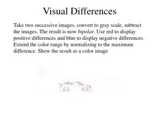
Visual Differences. Take two successive images, convert to gray scale, subtract the images. The result is now bipolar . Use red to display positive differences and blue to display negative differences.

E N D
Visual Differences Take two successive images, convert to gray scale, subtract the images. The result is now bipolar. Use red to display positive differences and blue to display negative differences. Extend the color range by normalizing to the maximum difference. Show the result as a color image
bipolar_image function rgb = bipolar_image(im) % % display bipolar differences as blue -> red scale r = ones(size(im)); g = r; b = r; idx = find(im>0); g(idx) = 1 - im(idx); b(idx) = g(idx); idx = find(im<0); g(idx) = 1 + im(idx); r(idx) = g(idx); rgb = cat(3,r,g,b); imshow(rgb);
Script – generate the movie nframes = length(seq); mov = avifile('test.avi','fps',5); im1 = im2double(rgb2gray(seq(1).cdata)); for n=2:nframes im2 = im2double(rgb2gray(seq(n).cdata)); rgb = bipolar_image(im2-im1); im1 = im2; fr = im2double(rgb/max(rgb(:))); mov = addframe(mov,fr); end mov = close(mov);
Mobile Sequence s(x,y) sx(x,y) sy(x,y) st(x,y)
Result of OptFlow Elapsed time is 103.172000 seconds.
Result of HSOptFlow Elapsed time is 0.312000 seconds.
Test Cases I tried two test cases. The first had a simple ramp in the horizontal direction that moves horizontally. The block search algorithm fails because of the aperture effect. There is no unique minimum. The second uses a quadratic circular pattern that moves two pixels to the left. These are contour plots of the two images superimposed on one plot. blue = before red = after
Matlab Script for Test Case x = linspace(-0.6,0.6,80); im = ones(size(x))'*x; im1 = im.^2+(im').^2; rgb = cat(3,im1,im1,im1); seq(1)=im2frame(rgb); dx = x(2)-x(1); im2 = (im+2*dx).^2 + (im').^2; rgb = cat(3,im2,im2,im2); seq(2)=im2frame(rgb); clear rgb;
OptFlow on Test Case >> [us vs] = OptFlow(seq,1); Elapsed time is 6.235000 seconds.
OptFlow on Test Case >> [us vs] = OptFlow(seq,1); Elapsed time is 6.235000 seconds. >> idx = 8:12; >> vs(idx,idx) ans = -2.0000 -2.0000 -2.0000 -2.0625 -2.0000 -2.0000 -2.0000 -2.0000 -2.0000 -2.0000 -2.0000 -2.0000 -1.9375 -2.1250 -2.0000 -2.0000 -2.0000 -2.0625 -2.0000 -2.0000 -2.0000 -2.0000 -2.0000 -2.0000 -2.0000 >> us(idx,idx) ans = 0 0 0 0 0 0 0 0 0 0 0 0 -0.0625 -0.0625 0 -0.0625 0 -0.1250 -0.1250 0 0 0 0 0 0
Modified Block Search I modified the block search routine to work like Matlab image processing toolbox blkproc operations. >> [vx vy] = blocks(im1,im2,[5 5],[5 5]); Elapsed time is 0.469000 seconds.
New Block Processer >> idx = 8:12; >> vx(idx,idx) ans = -2 -2 -2 -2 -2 -2 -2 -2 -2 -2 -2 -2 -2 -2 -2 -2 -2 -2 -2 -2 -2 -2 -2 -2 -2 >> vy(idx,idx) ans = 0 0 0 0 0 0 0 0 0 0 0 0 0 0 0 0 0 0 0 0 0 0 0 0 0
HSOptFlow on Test Case The result is strange until you look at the contour and realize that HS really is calculating localized normal flow. >> [us vs] = HSOptFlow(seq,1); dsx1 max 0.0176471 dsx2 max 0.0156863 Elapsed time is 0.203000 seconds.
Results of Lucas-Kanade Method >> [vx vy] = LKOptFlow(im1,im2,[5 5],[0 0]); Elapsed time is 0.016000 seconds.
LK Method – Numerical Results >> idx=8:12; >> vx(idx,idx) ans = -2.0000 -2.0000 -2.0000 -2.0000 -2.0000 -2.0000 -2.0000 -2.0000 -2.0000 -2.0000 -2.0000 -2.0000 -2.0000 -2.0000 -2.0000 -2.0000 -2.0000 -2.0000 -2.0000 -2.0000 -2.0000 -2.0000 -2.0000 -2.0000 -2.0000 >> vy(idx,idx) ans = 1.0e-013 * -0.0082 -0.0208 0.0729 0.1497 0.0504 0.0095 0.0339 -0.0919 -0.1461 -0.0994 0.0038 -0.0099 -0.1725 0 -0.1731 0.0034 0.0142 -0.0946 -0.4395 -0.2779 -0.0025 0.0054 -0.2432 0 0.2152
Block Search (mobile Frames 1,2) >> [vx vy] = blocks(im1,im2,[5 5],[5 5]); Elapsed time is 5.703000 seconds.
Average Motion (Block Search) 210-1-2 0.0006 0.0009 0.0023 0.0018 0.0006 0.0009 0.0035 0.0079 0.0035 0.0021 0.0041 0.0106 0.1268 0.6954 0.0176 0.0041 0.0029 0.0091 0.0211 0.0023 0.0006 0.0012 0.0035 0.0035 0.0012 -2 -1 0 1 2 70% of the image shifted 1 pixel right
HSOptFlow (revised) mobile frames 1 & 2 Algorithm revised from handout – changed alpha2 and iteration count.
Distribution of Velocities Velocity not tightly clustered. The average flow is to the right less than 0.5 pixel vxc = vx(:); vyc = vy(:); plot(vxc,vyc,'.');
Lucas-Kanade mobile frames 1 & 2
Time Difference after Registration >> diff = im2(:,2:352)-im1(:,1:351); >> dmax = max(abs(diff(:))); >> rgb = bipolar_image(diff/dmax);
LK Pan (upper-left quadrant) mobile frames 1 & 2 >> mean(mean(vx(1:20,1:20))) ans = 1.1088 >> mean(mean(vy(1:20,1:20))) ans = 0.1153
Register Images (fractional shift) dx = 1.11; dy=.11; T = maketform('affine',[1 0 0; 0 1 0; dx dy 1]); [nr nc] = size(im1); out = imtransform(im1,T,'XData',[1 nc],'YData',[1 nr]); diff = im2 - out; rgb = bipolar_image(diff);
mobile Frames 1 and 5 >> [vx vy] = blocks(im1,im2,[5 5],[5 5]); Elapsed time is 5.781000 seconds. >> mean(mean(vx(5:10,5:10))) ans = 4.9722 >> mean(mean(vy(5:10,5:10))) ans = 0.9722
Register Frames no pan pan (5,0) Simple pan is not registering the static background completely. pan (5,1)
Pan Registration Script dx = 5; dy=1; T = maketform('affine',[1 0 0; 0 1 0; dx dy 1]); [nr nc] = size(im1); [out,xdata,ydata] = imtransform(im1,T,'XData',[1 nc],'YData',[1 nr]); diff = im2 - out; rgb = bipolar_image(diff);
Color Velocity Encode hue as direction of motion and saturation as magnitude of motion. Let value = 1. function rgb = color_velocity(vx,vy) sat = sqrt(vx.^2+vy.^2); value = ones(size(sat)); hue = angle(vx+j*vy)/pi; hue = hue(:); idx = find(hue<0); hue(idx) = 2+hue(idx); hue = hue/2; hue = reshape(hue,size(sat)); rgb = hsv2rgb(hue,sat,value); imshow(rgb);
Mobile Frames 1 & 2 color velocity map Frame 2
Pan Compensation before after
Matlab Script load mobile_short im1 = rgb2gray(im2double(seq(1).cdata)); im2 = rgb2gray(im2double(seq(2).cdata)); [vx vy] = LKOptFlow(im1,im2,[5 5],[0 0]); rgb = color_velocity(vx,vy); imwrite(rgb,'color_velocity1.jpg'); script3 % pan compensation script [vx2 vy2] = LKOptFlow(out,im2,[5 5],[0 0]); rgb2 = color_velocity(vx2,vy2); imwrite(rgb2,'color_velocity2.jpg');