Download
1 / 22
220 likes | 301 Views
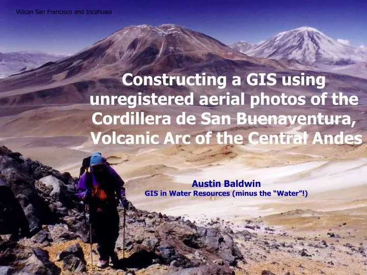
Volcan San Francisco and Incahuasi. Constructing a GIS using unregistered aerial photos of the Cordillera de San Buenaventura, Volcanic Arc of the Central Andes Austin Baldwin GIS in Water Resources (minus the “Water”!). 22,590 ft. Nevado Ojos del Salado, Argentina/Chile border.

E N D
Volcan San Francisco and Incahuasi Constructing a GIS using unregistered aerial photos of the Cordillera de San Buenaventura, Volcanic Arc of the Central Andes Austin Baldwin GIS in Water Resources (minus the “Water”!)
22,590 ft. Nevado Ojos del Salado, Argentina/Chile border 14,760 ft.
Objectives: • Create a GIS of the Cordillera de San Buenaventura using: • Roads and International Borders • GTOPO30 Topography • Landsat Satellite Imagery • Rock Sample Waypoints • 2. Add unregistered aerial photos to the GIS
Roads and International Borders: Downloaded from the ESRI Geography Network website http://www.geographynetwork.com
GTOPO30 Topographic Information: Downloaded from the USGS website. http://edcdaac.usgs.gov/gtopo30/gtopo30.html
Landsat Satellite Imagery: Downloaded from NASA’s MrSID website. https://zulu.ssc.nasa.gov/mrsid/
Rock Sample Waypoints: 50 rock samples were collected in the field, and their locations were recorded using a GPS receiver.
Rock Sample Waypoints: 50 rock samples were collected in the field, and their locations were recorded using a GPS receiver.
N ? N ? PART II: Adding aerial photos to the GIS • Problems: • not orientated in • compass directions • not georegistered • unknown scale • geographic • distortion 1 km or 100 km?
Adding aerial photos to the GIS: Why Bother?? Digitizing Surface Features: Air photo resolution is far superior to other imagery sources, such as Landsats or topographic maps. This high resolution reveals surface features such as faults which may be impossible to distinguish in Landsats. With georegistered air photos, these features could be digitized as a layer in ArcMap. Field Mapping: In the field, knowledge of scale, map orientation, and Easting/Northing is very useful.
Resolution Comparison between Landsat imagery and air photo Aerial Photo Satellite Landsat image
Another Resolution Comparison Satellite Landsat image Aerial Photo
Adding aerial photos to the GIS: The Georeferencing tool allows the user to align- or georeference- data without a coordinate system (i.e., air photos) to a map with a coordinate system. It is essential that there are physical features visible in the existing map that are also visible in the air photo. For example, road intersections, buildings, or mountain peaks. These common features will be used to “link” the air photo to the map.
Adding aerial photos to the GIS: Start by adding the unregistered air photo to the data frame containing the existing map. On the Georeferencing toolbar, select ‘Fit to Display’ to bring the air photo into the field of view with the Landsat.
Making a Link between a common feature: Using the ‘Add Control Points’ tool, make a link between a feature common to both the air photo and the registered data. Click a point on the air photo first, then on the registered data.
Select the Transformation (aka, “rubberization”): The Transformation Order controls how much the new data will be distorted for a best fit of the links. 1st Order Polynomial (Affine): To shift, scale, and rotate the image. Only for images with no geographic distortion- Requires 3 links for an exact match. 2nd Order Polynomial: Allows some pull and stretch of the image. Requires at least 6 links. 3rd Order Polynomial: Allows maximum amount of stretch and pull of the image for a best fit of the links. Used for images with considerable distortion. Requires at least 10 links.
How well do they match? Aerial Photo Georegistered Landsat image
Air Photo Landsat image
Final Product: High-resolution, georegistered aerial photographs, ready for digitizing or field mapping!
Limitations of this method: • Must have a georegistered layer for linking common points. • Resolution of images- with coarse resolution it is more difficult to pinpoint common locations for linking. • Geometric Distortion of aerial photos- makes it impossible to align all points. “Orthophotos” correct for this distortion, but are costly.
Muchas Gracias! Laguna Miscanti, northern Chile