Download
1 / 24
240 likes | 384 Views
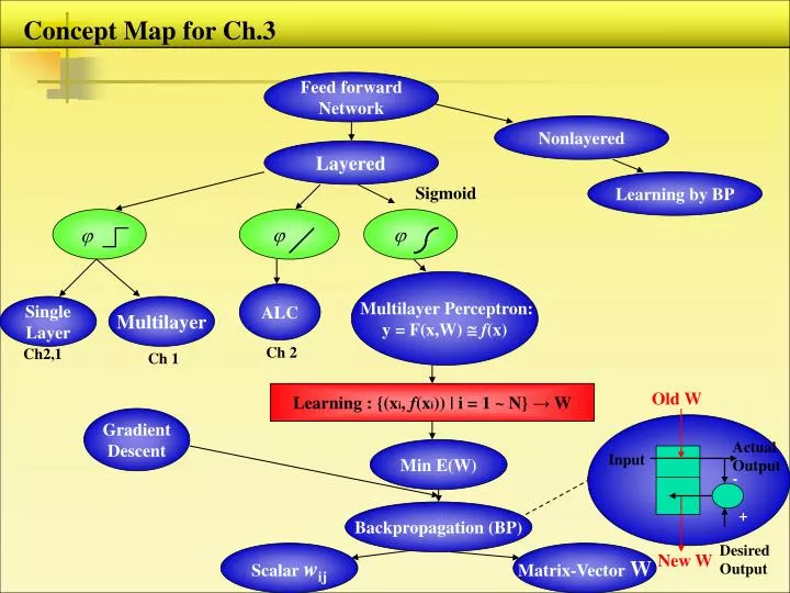
Concept Map for Ch.3. Feed forward Network. Nonlayered. Layered. Learning by BP. Sigmoid. . . . Multilayer Perceptron: y = F(x,W) f (x). ALC. Single Layer. Multilayer. Ch 2. Ch2,1. Ch 1. Learning : {(x i , f (x i )) | i = 1 ~ N} → W. Old W. Gradient Descent.

E N D
Concept Map for Ch.3 Feed forward Network Nonlayered Layered Learning by BP Sigmoid Multilayer Perceptron: y = F(x,W) f(x) ALC Single Layer Multilayer Ch 2 Ch2,1 Ch 1 Learning : {(xi, f(xi)) | i = 1 ~ N} → W Old W Gradient Descent Actual Output Min E(W) Input - Backpropagation (BP) + Desired Output Scalar wij Matrix-Vector W New W
Chapter 3. Multilayer Perceptron • MLP Architecture – Extension of Perceptron to Many layers and Sigmoidal Activation functions • – for real-valued mapping/classification
Learning: Discrete → Find W* → Continuous F(x, W*) f(x)
u j S u j 1 0 -1 1 Smaller 0 Logistic Hyperbolic Tangent
2. Weight Learning Rule – Backpropagation of Error • Training Data ( )Weights (W): • Curve (Data) Fitting (Modeling, NL Regression) NN Approximating Function True Function (2) Mean Squared Error E for 1-D function as an Example
0 , n Number of Iterations (3) Gradient Descent Learning (4) Learning Curve E{ W(n), weight track } E 0 Iteration = One scan of the training set (Epoch)
d - d ( d y ) y y j k k k j i u u u y w w j i k k j j j ij jk (5) Backpropagation Learning Rule Features: Locality of Computation, No Centralized Control, 2-Pass xi B. Inner Layer Weights A. Output Layer Weights where where (Credit assignment)
Water Flow Analogy to Backpropagation ( DropObject Here ) River Flow w1 Input - Many weights (Flows) - Flow wl If the error is very sensitive to a weight change, then change that weight a lot, and vice versa. → Gradient Descent , Minimum Disturbance Principle ( Fetch Object Here ) Output
No desired response is needed for hidden nodes. must exist = sigmoid [tanh or logistic] For classification, d = ± 0.9 for tanh, d = 0.1, 0.9 for logistic. h (6) Computation Example : MLP(2-1-2) A. Forward Processing : Comp. Function Signals
sum = - v w e d y 21 1 1 1 1 1 sum 1 h sum 22 = - v w e d y 2 2 2 2 2 B. Backward Processing - Comp. Error Signals has been computed in forward processing
If we knew f(x,y), it would be a lot faster to use it to calculate the output than to use the NN.
Student Questions: Does the output error become more uncertain in case of complex multilayer than simple layer ? Should we use only up to 3 layers ? Why can oscillation occur in the learning curve ? Do we use the old weights for calculating the error signal δ ? What does ANN mean ? Which makes more sense, error gradient or the weight gradient considering the equation for weight change ? What becomes the error signal to train the weights in forward mode ?