Download
1 / 36
360 likes | 519 Views
Proving Non-Reconstruction on Trees by an Iterative Algorithm. Elitza Maneva University of Barcelona joint work with N. Bhatnagar, Hebrew University. ?. 2435 1026 324. 2 0 1. 0 1 0. 1 0 1. 0 1 1. Optimal Algorithm for Reconstruction: Belief Propagation

E N D
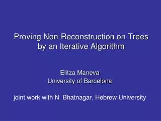
Proving Non-Reconstruction on Trees by an Iterative Algorithm Elitza Maneva University of Barcelona joint work with N. Bhatnagar, Hebrew University
2435 1026 324 2 0 1 0 1 0 1 0 1 0 1 1 Optimal Algorithm for Reconstruction: Belief Propagation computes the distribution at the root given the boundary
Random variable LR(n) : colors at vertices at level n. For what degree is limn E[Pr[R at the root | LR(n)]] = 1/q ?
Total variation distance: dTV(, )=1/2 L D |(L)-(L)| Random variable LR(n) : colors at vertices at level n. For what degree is limndTV (LR(n), LG(n)) = 0 ?
Interest in reconstruction (in chronological order) • Probability: Extremality of the free-boundary Gibbs measure (since 1960s) • Phylogeny: reconstructing ancestry tree of collection of species • Physics: Replica symmetry breaking (dynamical transition) in spin-glasses • Computer Science: Glauber dynamics, MCMC, message-passing algorithms
0 Space of solutions of random Constraint Satisfaction Problems n variables dn constraints are chosen at random Unsat Easy Hard dr ds d
limndTV (LR(n), LG(n)) = 0 Tree: Random graph:
limndTV (LR(n), LG(n)) = 0 limndTV (LR(n), LG(n)) > 0 Tree: Random graph:
limndTV (LR(n), LG(n)) = 0 limndTV (LR(n), LG(n)) > 0 Tree: Random graph: Conjecture
Other models • Potts model: q colors, parameter [0,1] color of child node = same as parent’s color with prob. every other color with prob. (1- )/(q-1) • Asymmetric channels: q colors, qq matrix M Mi, j= Prob [child gets color j | parent is color i] • Same on Galton-Watson trees (i.e. random degrees) • 3-SAT: 0 x1 x3 x2 x4 x5 1 1 0 1
RSB, clustering of solutions and reconstruction highlights • [Mezard-Parisi-Zechina ‘03] Survey Propagation algorithm and satisfiability threshold calculation for 3-SAT and coloring, based on Replica Symmetry Breaking Ansatz. • [Mezard-Montanari ‘06] The dynamic replica symmetry breaking threshold is the same as the threshold for reconstruction on the tree. • [Achlioptas--Coja-Oghlan ‘08] For sufficiently large q, there exists a sequence q 0 s.t. the space of colorings is clustered for random graphs of average degree (1+q) q log q < d < (2- q) q log q. • [Sly ‘08] For sufficiently large q: q (log q + log log q + 1 - ln 2 -o(1)) < dr < q (log q + log log q + 1+o(1))
RSB, clustering of solutions and reconstruction highlights • [Mezard-Parisi-Zechina ‘03] Survey Propagation algorithm and satisfiability threshold calculation for 3-SAT and coloring, based on Replica Symmetry Breaking Ansatz. • [Mezard-Montanari ‘06] The dynamic replica symmetry breaking threshold is the same as the threshold for reconstruction on the tree. • [Achlioptas--Coja-Oghlan ‘08]For sufficiently large q, there exists a sequence q 0 s.t. the space of colorings is clustered for random graphs of average degree (1+q) q log q < d < (2- q) q log q. • [Sly ‘08]For sufficiently large q: q (log q + log log q + 1 - ln 2 -o(1)) < dr < q (log q + log log q + 1+o(1))
Easy lower bound by coupling dreconstruction > q-1
Upper bound: boundary forcing the root dreconstructionsoln(∑ (-1)j()(q-1-jx)d /(q-1)d = x) q-1 j=0 q-1 j
The bounds for coloring • [Zdeborova-Krzakala ‘07] • Heuristic algorithm for computing threshold for general models • Heuristic analysis predicted the asymptotic result of Sly • [Sly ‘08][Bhatnagar-Vera-Vigoda ‘08]For q sufficiently large: Hard step (need large q): After sufficiently many iterations dTV < 2/q. Easy step: Given that dTV< 2/q, dTV goes to 0. • [Bhatnagar-Maneva ‘09] • Rigorous algorithm for getting upper bounds on dTV for general models • Concrete bounds on the threshold for Potts model with small q.
2435 1026 324 2 0 1 0 1 0 1 0 1 0 1 1 BP: recursion on the distribution at the root given the boundary Here we need: Recursion on the distribution over possible distributions at the root when the boundary is chosen at random.
Some notation 2435 1026 324 1 2,… d f:(Rq)d Rq f i(1 2,…, d) = t=1 (ji tj) |||| = i i d
Recursion on the tree depth QGn random q-dim vector QGn (R) := Prob[R|L], where L~ LG(n) Pr[QGn+1 = ] = 1/(q-1)d Pr [f(Qc1n, …, Qcdn) ] c1,.., cd {1,..,q}\G
Population dynamics Pr[QGn+1 = ] = 1/(q-1)d Pr [f(Qc1n, …, Qcdn) ] • Keep “populations” of N samples each from the distributions of QRn, QGn, …etc. • Generating the population of QGn+1: • Choose d colors c1, …, cd from {1, …, q}\G independently • Choose 1, …,d randomly respectively from the populations for Qc1n, …, Qcdn • Save f(1, …,d )/||f(1, …,d )|| into the population for QGn+1 c1,..,cd {1,..,q}\G
Recursions on the tree depth • Conditional recursion: QGn random q-dim vector QGn (R) := Prob[R|L], where L~ LG(n) Pr[QGn+1 = ] = 1/(q-1)d Pr [f(Qc1n, …, Qcdn) ] • Unconditional recursion: Qn random q-dim vector Qn(R) := Prob[R|L], L is a random boundary Pr[Qn+1= ] E[ ||f(Qn(1),…, Qn(d))|| Ind[ f(Qn(1),…,Qn(d)) ] c1,.., cd {1,..,q}\G
Discrete surveys algorithm Pr[Qn+1= ] E[ ||f(Qn(1),…, Qn(d))|| Ind[f(Qn(1),…, Qn(d)) ] • Keep a “survey” of the distribution of Qn • Generate the survey of Qn+1 by applying the recursion to the survey of Qn. 1 distrib. of Qn R 0.25 0.05 0.11 0.08 0 1 G
Discrete surveys algorithm Pr[Qn+1= ] E[ ||f(Qn(1),…, Qn(d))|| Ind[f(Qn(1),…, Qn(d)) ] • Keep a “survey” of the distribution of Q_n • Generate the survey of Qn+1 by applying the recursion to the survey of Qn. 1 1 distrib. of Qn survey of Qn R R 0.25 0.05 0.11 0.08 0 1 0 1 G G
Definition of a discrete survey • Let P be the space of q-dim probability vectors. • Let S= (S1, …, Sk) P and convex hull of S is <S> • Let 1, … k be functions i:<S>[0,1], s.t for every <S>: 1. ii () =1 2. = ii() Si ( define a convex decomposition of ). • Let P be a random element of P with support in <S>. • Let C be a random element of S with Pr[C=Si] = E[i(P)]. • Then we say that C is a survey of P on the skeleton (S, 1, … k)
Properties of discrete surveys • Transitivity: If C is a survey of P and D is a survey of C then D is a survey of P. • Mixing: If C1, C2 are surveys respectively of P1 and P2 then the r. v. with distribution the mixture p C1+(1-p) C2 is a survey of the r.v. with distribution p P1+(1-p) P2. • For any multi-affine function f : PdP, if C1, …, Cd are surveys of P1, …, Pd then the r.v. D defined by Pr[D=] E[ ||f(C1, …, Cd)|| x Ind [f(C1, …, Cd) ]] is a survey of the r.v. Q defined by Pr[Q=] E[ ||f(P1, …, Pd)|| x Ind [f(P1, …, Pd) ]] • For a convex function g on P, if C is a survey of P then E[g(P)] ≤ E[g(C)].
Manual part of the algorithm • Selection of skeletons of small size k • complexity of the algorithm: O(nkd) • k generally needs to be exponential in q • the skeleton can be refined progressively • Examples on Potts model: • q=3, d=3, =0n=14, k=19 was enough • q=3, d=2, =0.79n<100, k≤208 was enough • q=3, d=3, =0.7n<100, k≤85 was enough • q=3, d=2 or 3, =0.74n<100, k≤61 was enough
A proof that dTV is small implies dTV 0 • There is no general strategy • For Potts model, due to [Sly ‘09]: xn:= EL~L (n)[Prob[R|L]-1/q]= q EL [ (Prob[R|L]-1/q)2] we have xn+1 ≤ d2xn+ c2(q,d,) xn2 +… +cd(q,d,) xnd • Thus we could find >0 and c<1 such that if xn< then xn+1 < c xn R
Bound of Formentin and Külske ‘09 • α: stationary vector of positive matrix M • S(p|α) := Σip(i) log( p(i)/α(i) ) • L(p) := S(p|α) + S(α|p) • Mrev(i,j) := α(j) M(j, i)/α(i) • c(M):= supp L(pMrev)/L(p) Theorem: If E[d] c(M) < 1 then no reconstruction.
Important Questions • For the Potts model better bounds were obtained by [Formentin-Külske ‘09]. Could they be tight? Can their method be generalized to models with hard constraints? • The design of the Survey Propagation algorithm also includes a discretization step - could this step be done in a controlled manner too? • How are reconstruction on trees and clustering of solutions related?
[Mezard, Montanari `05] The dynamical transition at d correspond to the phase transition for reconstruction on the tree.
[Mezard, Montanari `05] The dynamical transition at d correspond to the phase transition for reconstruction on the tree.
[Mezard, Montanari `05] The dynamical transition at d correspond to the phase transition for reconstruction on the tree. ?
[Allan Sly `08] For q-coloring: d≤ q(log q + log log q + 1 + o(1)) (also [Zdeborova, Krzakala ’07]) d ≥ q(log q + log log q + 1 – ln 2 –o(1)) For constant q it is open. Estimates can be obtained with population dynamics.
What phenomena on the tree are described by the other transitions? • Can we make population dynamics official? Find rigorous approximations for it? (it would imply that 4.267 is an upper bound in the threshold by the results of [Franz, Leone `03] and [Talagrand Panchenko `03]) • About clustering: is “phase” and “cluster” really the same thing?