Download
1 / 59
590 likes | 799 Views
Combinatorial Pattern Matching. Outline. Microarrays and Introduction to Clustering Hierarchical Clustering K-Means Clustering Corrupted Cliques Problem CAST Clustering Algorithm . Section 1: Microarrays and Introduction to Clustering. What Is Clustering?.

E N D
Outline • Microarrays and Introduction to Clustering • Hierarchical Clustering • K-Means Clustering • Corrupted Cliques Problem • CAST Clustering Algorithm
What Is Clustering? • Viewing and analyzing vast amounts of biological data can be perplexing. • Therefore it is easier to interpret the data if they are partitioned into clusters combining similar data points.
Inferring Gene Functionality • Researchers want to know the functions of newly sequenced genes. • Simply comparing new gene sequences to known DNA sequences often does not give away the function of gene. • For 40% of sequenced genes, functionality cannot be ascertained by only comparing to sequences of other known genes. • Microarrays allow biologists to infer gene function even when sequence similarity alone is insufficient to infer function.
Microarrays and Expression Analysis • Microarrays: Measure the expression level of genes under varying conditions/time points. • Expression level is estimated by measuring the amount of mRNA for that particular gene. • A gene is active if it is being transcribed. • More mRNA usually indicates more gene activity.
How do Microarray Experiments Work? • Produce cDNA from mRNA (DNA is more stable). • Attach phosphor to cDNA to determine when a particular gene is expressed. • Different color phosphors are available to compare many samples at once. • Hybridize cDNA over the microarray. • Scan the microarray with a phosphor-illuminating laser. • Illumination reveals transcribed genes. • Scan microarray multiple times for the differently colored phosphors.
Microarray Experiments Phosphors can be added here instead Instead of staining, laser illumination can be used www.affymetrix.com
Using Microarrays • Track the sample over a period of time to see gene expression over time. • Each box on the right represents one gene’s expression over time.
Using Microarrays: Example • Green: Expressed only from control. • Red: Expressed only from experimental cell. • Yellow: Equally expressed in both samples. • Black: NOT expressed in either control or experimental cells. Sample Microarray
Interpreting Microarray Data • Microarray data are usually transformed into an intensity matrix (below). • The intensity matrix allows biologists to find correlations between different genes (even if they are dissimilar) and to understand how genes’ functions might be related. • Each entry contains theintensity (expression level)of the given gene at themeasured time.
Applying Clustering to Microarray Data • Plot each datum as a point in N-dimensional space. • Create a distance matrix for the distance between every two gene points in the N-dimensional space. • Genes with a small distance share the same expression characteristics and might be functionally related or similar. • Therefore, clustering “close” genes together reveals groups of functionally related genes.
Clustering: Example Clusters
Homogeneity and Separation Principles • Every “good” clustering must have two properties: • Homogeneity: Elements within the same cluster are close to each other. • Separation: Elements in different clusters are located far from each other.
Homogeneity and Separation Principles • Every “good” clustering must have two properties: • Homogeneity: Elements within the same cluster are close to each other. • Separation: Elements in different clusters are located far from each other. • Therefore clustering is not an easy task!
Homogeneity and Separation Principles • Every “good” clustering must have two properties: • Homogeneity: Elements within the same cluster are close to each other. • Separation: Elements in different clusters are located far from each other. • Therefore clustering is not an easy task! • Example: Two (of many) clusterings:
Homogeneity and Separation Principles • Every “good” clustering must have two properties: • Homogeneity: Elements within the same cluster are close to each other. • Separation: Elements in different clusters are located far from each other. • Therefore clustering is not an easy task! • Example: Two (of many) clusterings: • BAD (Homogeneity? Separation?)
Homogeneity and Separation Principles • Every “good” clustering must have two properties: • Homogeneity: Elements within the same cluster are close to each other. • Separation: Elements in different clusters are located far from each other. • Therefore clustering is not an easy task! • Example: Two (of many) clusterings: • BAD (Homogeneity? Separation?) • GOOD
Three Primary Clustering Techniques • Agglomerative: Start with every element in its own cluster, and iteratively join clusters together. • Divisive: Start with one cluster and iteratively divide it into smaller clusters. • Hierarchical: Organize elements into a tree. • Leaves represent genes. • Path lengths between leaves represent the distances between genes. • Similar genes therefore lie within the same subtree.
Hierarchical Clustering and Evolution • Hierarchical Clustering can be used to reveal evolutionary history.
Hierarchical Clustering Algorithm • Hierarchical Clustering (d, n) • Form n clusters each with one element • Construct a graph T by assigning one vertex to each cluster • while there is more than one cluster • Find the two closest clusters C1 and C2 • Merge C1 and C2 into new cluster C with |C1| +|C2| elements • Compute distance from C to all other clusters • Add a new vertex C to T and connect to vertices C1 and C2 • Remove rows and columns of d corresponding to C1 and C2 • Add a row and column to d corresponding to new cluster C • return T • The algorithm takes an nxn distance matrix d of pairwise distances between points as an input.
Hierarchical Clustering Algorithm • Hierarchical Clustering (d, n) • Form n clusters each with one element • Construct a graph T by assigning one vertex to each cluster • while there is more than one cluster • Find the two closest clusters C1 and C2 • Merge C1 and C2 into new cluster C with |C1| +|C2| elements • Compute distance from C to all other clusters • Add a new vertex C to T and connect to vertices C1 and C2 • Remove rows and columns of d corresponding to C1 and C2 • Add a row and column to d corresponding to new cluster C • return T • The algorithm takes an nxn distance matrix d of pairwise distances between points as an input. • Different notions of “distance” give different clusters.
Hierarchical Clustering: Two Distance Metrics • Minimum Distance: • Here the minimum is taken over all x in C and all y in C*. • Average Distance: • Here the average is also taken over all x in C and all y in C*.
Squared Error Distortion • Given a data point v and a set of points X, define the distance from v to X, d(v, X) as the (Euclidean) distance from v to the closestpoint inX. • Given a set of n data points V = {v1…vn} and a set of k points X, define the Squared Error Distortion as
K-Means Clustering Problem: Formulation • Input: A set V consisting of n points and a parameter k • Output: A set X consisting of k points (cluster centers) that minimize the squared error distortion d(V, X) over all possible choices of X.
An Easy Case: k = 1 • Input: A set, V, consisting of n points • Output: A single point x (cluster center) that minimizes the squared error distortion d(V, x) over all possible choices of x.
An Easy Case: k = 1 • Input: A set, V, consisting of n points • Output: A single point x (cluster center) that minimizes the squared error distortion d(V, x) over all possible choices of x. • The 1-means clustering problem is very easy. • However, it becomes NP-Complete for more than one center (i.e. k > 1). • An efficient heuristic for the case k > 1 is Lloyd’s Algorithm.
K-Means Clustering: Lloyd’s Algorithm • Lloyd’s Algorithm • Arbitrarily assign the k cluster centers • while the cluster centers keep changing • Assign each data point to the cluster Cicorresponding to the closest cluster representative (center) (1 ≤ i ≤ k) • After the assignment of all data points, compute new cluster representatives according to the center of gravity of each cluster, that is, the new cluster representative for each cluster C is Note: This may lead to only a locally optimal clustering.
x1 x2 x3 Lloyd’s Algorithm: Illustration
x1 x2 x3 Lloyd’s Algorithm: Illustration
x3 x2 x1 Lloyd’s Algorithm: Illustration
x1 x2 x3 Lloyd’s Algorithm: Illustration
x1 x2 x3 Lloyd’s Algorithm: Illustration
Conservative K-Means Algorithm • Lloyd’s algorithm is fast, but in each iteration it moves many data points, not necessarily causing better convergence. • A more conservative greedy method would be to move one point at a time only if it improves the overall clustering cost • The smaller the clustering cost of a partition of data points, the better that clustering is. • Different methods (e.g., the squared error distortion) can be used to measure this clustering cost.
K-Means “Greedy” Algorithm • ProgressiveGreedyK-Means(k) • Select an arbitrary partition P into k clusters • while forever • bestChange 0 • for every cluster C • for every element i not in C • if moving i to cluster C reduces its clustering cost • if (cost(P) – cost(Pi C) > bestChange • bestChange cost(P) – cost(Pi C) • i*I • C* C • ifbestChange > 0 • Change partition P by moving i* to C* • else • returnP Note: We are free to change how the clustering cost is calculated.
Clique Graphs • A clique in a graph is a subgraph in which every vertex is connected to every other vertex. • A clique graph is a graph in which each connected component is a clique. • Example: This clique graph is composed of three cliques.
Transforming Any Graph into a Clique Graph • A graph can be transformed into a clique graph by adding or removing edges. • Example:
Transforming Any Graph into a Clique Graph • A graph can be transformed into a clique graph by adding or removing edges. • Example: