Download
1 / 25
260 likes | 429 Views
The Use of Multivariate Analysis Techniques to Design a Class Plan. 1999 CAS Seminar on Ratemaking. Overview of Presentation. Background Multivariate analysis techniques: Generalized Linear Models (GLMs) Classification and Regression Trees (CART,CHAID) Implementation Pricing Marketing

E N D
The Use of Multivariate Analysis Techniques to Design a Class Plan 1999 CAS Seminar on Ratemaking Mark Scully, Tillinghast-Towers Perrin
Overview of Presentation • Background • Multivariate analysis techniques: • Generalized Linear Models (GLMs) • Classification and Regression Trees (CART,CHAID) • Implementation • Pricing • Marketing • Agents’ compensation • Results monitoring
Several Factors are Converging toward Better Analysis of Customer and Prospect Attributes • Greater emphasis on pricing vs. underwriting • Increased familiarity with techniques • Faster computers • Influence of direct writers, non-standard cos.and banks • Use of multiple distribution channels • Increased competition
Why Multivariate Statistical Techniques? • Most rating variables are correlated. • Different variables may be showing the same underlying effect. • Repeated use of univariate techniques leads to double-counting of same effects. • Can capture interactions. • Provides more than a point estimate, also standard errors.
Annual Mileage Driving Intensity Vehicle Make/Model Driver Age Different Rating Variables may be Manifestations of the Same Underlying Effect Underlying Effect Rating Variables
Interactions Arise when the Combined Effect of two Variables Differs from the Sum of their Single Effects The differential between female and male differs by age.
Confidence Intervals Indicate the Degree of Certainty Inherent in Relativity Estimates
Confidence Intervals Indicate the Degree of Certainty Inherent in Relativity Estimates
Confidence Intervals Indicate the Degree of Certainty Inherent in Relativity Estimates
Statistical Rating Techniques Indicate the Relative Explanatory Power of each Variable... Variable B Variable A …and the extent to which variables are correlated.
What statistical techniques do we commonly use? • Generalized Linear Models (GLMs) • Classification and regression trees • CHAID • CART
What are GLMs? • Statistical procedure for measuring the effect of one or more independent variables upon a dependent variable • Dependent variables are, for ratemaking, typically: • frequency and • severity • GLMs allow extreme flexibility in model structure and design • multiplicative or additive plans (or others) • different error distributions • variable interactions • Explicitly produce relativity estimates (and more)
Basic Theory of GLMs (I) Let Yi, I=1,2,…,n be observations from a random variable. We model them as follows: • Where: • h=the link function • xi=a vector of variables associated with the i-th observation • I=a scalar parameter (the offset) • =the parameter vector • ei=an error term(with mean equal to 0)
Basic Theory of GLMs (II) Typically, the random term ei is chosen from the exponential family with density in the following general form: Where and are parameters and w the weight of each observation. If we denote the mean of this distribution as then its variance may be expressed as V() /w, where V(•) is referred to as the variance function.
Literature on GLMs • Generalized Linear Models, Second Edition, P. McCullach and J.A. Nelder, Chapman & Hall 1989 (ISBN 0 412 31760 5) • “Statistical Motor Rating: making Effective Use of Your Data”, M.J. Brockman and T.S. Wright, JIA 119, III, 457-543 (April 1992). • “Technical Aspects of Domestic Lines Pricing”, Greg Taylor, University of Melbourne Research Paper 45 (ISBN 0 7325 1474 6)
GLMs-Some Practical Considerations (I) • A log link function produces multiplicative relativities. • Separate models for frequency and severity: • Better understanding of data • Appropriate distributions exist • Typical error distributions for frequency: • Poisson/Quasi-Poisson • Negative binomial • Typical distributions for severity: • Normal • Gamma • Inverse Gaussian
GLMs-Some Practical Considerations (II) • Variables may be modeled as continuous covariates or categorical factors • An array of statistical and practical tests exists for model testing: • Variable significance tests • Quantile plots • Residual plots • Comparison of actual data to model
Comparison of Actual to Model Helps to Identify Areas Currently Under- or Overpriced Loss-Segments: How much do we write? Are we growing here? How many $ involved? Other reasons to stay here? Profit-Segments: How much do we write? Are we losing business? How many $ involved? How do we get more?
The Significance of these Profit/Loss Areas Depends also on their Volume of Business Note: Gain/(Loss) = (Current PP - Indicated PP) x Exposures
What are classification and regression trees? • Procedures for successively subdividing data into homogeneous groups • Like GLMs, they use a dependent variable and one or more independent ones • Result is not necessarily symmetric • Implicitly capture the natural interactions between factors • Can produce a simpler rating plan or form a single rating variable out of many • Produces homogeneous groups(i.e., a tree structure) but no rating plan or relativities
Classification and Regression Trees produce an asymmetrical grouping of the data Bestand SF M.O 1/2 SF 1-3 SF 5-10. SF 11-15 SF 15-22 11 Typ 10-15 Typ 16-20 Typ 21-25 Typ 10-17 Typ 18-25 Männlich. Weiblich Männlich Weiblich 3 6 9 10 12 13 Kfz-Alter < 2 Kfz-Alter > 2 Beamten R & A Garage Keine. 1 2 4 5 7 8
Some differences between CHAID and CART • Dependent variable for CHAID must be categorical; for CART it can be metric • Different splitting algorithm (e.g., CHAID uses a Chi-squared test using contingency tables) • CHAID splits into multiple groups, CART makes binary splits • Different stopping criteria
GLMS may be used to Produce a Rating Plan with Variables Generated by CART or CHAID Potential Rating Variables GLM Analysis CART/ CHAID Analysis CART/ CHAID Variables
Results from the Rating Analysis Can be Used Beyond the Production of a Rating Plan Rating Analysis Actuarially Optimal Model • Marketing • UW Guidelines • Agents’ Compensation • Monitoring • Constraints: • Regulatory • Agents • Stability • Competition • etc. Rating Plan Actually Implemented