Download
1 / 68
690 likes | 842 Views
Biological networks and statistical physics. Diego Garlaschelli. Dipartimento di Fisica, Università di Siena, ITALY. Said Business School, University of Oxford, UK. BioPhys09, Arcidosso, ITALY. Biological networks: from cells to ecosystems. Metabolic networks.

E N D
Biological networks and statistical physics Diego Garlaschelli Dipartimento di Fisica, Università di Siena, ITALY Said Business School, University of Oxford, UK BioPhys09, Arcidosso, ITALY
Biological networks: from cells to ecosystems
Metabolic networks Vertices = cellular substrates (products or educts) Links = biochemical reactions (enzyme-mediated) complex educt enzyme product educt (part of E. coli’s metabolic network )
Protein-protein interaction networks Vertices = proteins Links = interactions within the cell
Neural networks Vertices = neurons Links = synapses ← single neuron ↑ web of synaptic connections
Vascular networks Vertices = tissues Links = blood vessels 6 7 5 3 8 4 2 1
Ecological networks (food webs) Vertices = coexisting species Links = predator-prey interactions
Real networks versus regular graphs Protein-protein interaction network (Saccharomyces cerevisiae) Regular graphs Two problems: 1) characterization of network structure (and complexity) 2) network modelling
Graph Theory Undirected Graph Directed Graph “Graph”≡G(V,E) V: N vertices E: L links Adjacency Matrix: i j i i j j i j i i j j Degree(number of links) of vertex i corresponds to i j Average vertex-vertex distance: Clustering coefficient:
Large clustering coefficient C: “my friends are friends of each other” High robustness under vertex removal Small-world character of (most) real networks: Short mean distance D: “it’s a small world, after all!” Efficient information transport (and fast disease spreading too!)
Many poorly connected vertices Few highly connected vertices Degree distribution in (most) real networks: Power-law distribution P(k) k - 2<<3 No characteristic scale (scale-free)! (a) Archaeoglobus fulgidus (archea); (b) E. coli (bacterium); (c) Caenorhabditis elegans (eukaryote); (d) 43 different organisms together.
Finite-scale versus scale-free networks Finite-scale networks: P(k)decays exponentially No vertex has a degree much larger than the average value Scale-free networks: P(k) decays as a power law Few vertices have a degree much larger that the average value
5 vertices with largest degree vertices connected to the red ones(random 27%, scale-free 60%) other vertices Finite-scale versus scale-free networks Finite-scale networks: P(k)decays exponentially Scale-free networks: P(k) decays as a power law (in both cases N=130 and L=215: same average degree)
Degree distribution P(k): (Poisson) Average vertex-vertex distance: Clustering coefficient RANDOM GRAPH model (Erdös, Renyi 1959) ● Start with a set of N isolated vertices; ● For each pair of vertices draw a link with uniform probability p. p=0 p=0.1 p=0.5 p=1
Connected components in random graphs The interesting feature of the random graph model is the presence of a critical probabilitypc marking the appearance of a giant cluster: Percolation threshold pc 1/N When p<pc the network is made of many small clusters and P(s) decays exponentially; when p>pc there are few very small clusters and one giant one; at p=pc the cluster size distribution has a power-law form:P(s) s -
p=0 0<p<1 p = 1 P(k) 10 -1 10 -2 10 -3 10 -4 Regular Small-world Random Degree distribution C(p)/C(0) Average distance and clustering coefficient small-world regime D(p)/D(0) 0 4 8 12 16k SMALL-WORLD model (Watts, Strogatz Nature 1998) ● Start with a regular d-dimensional lattice, connected up to q nearest neighbours; ● With probability p, an end of each link is rewiredto a new randomly chosen vertex.
After a certain number of iterations, the degree distribution approaches a power-law distribution: P(k)k - =3 Growth and preferential attachment are both necessary! P(k)k - =3 SCALE-FREE model (Barabási, Albert Science 1999) ● Start with m0 vertices and no link; ● at each timestep add a a new vertex with m links, connected to preexisting vertices chosen randomly with probability proportional to their degree k (preferential attachment).
FITNESS model (Caldarelli et al.Phys. Rev. Lett. 2002) ● Each vertex i is assigned a fitness valuexi drawn from a given distribution r(x); ● A link is drawn between each pair of vertices i and j with probability f(xi,xj) depending on xi and xj . Power-law degree distributions are obtained by chosing r(x) x-α f(xi,xj) xi xj or r(x)= e-x f(xi,xj) (xi +xj –z)
1 2 5 6 3 4 Adjacency matrix (NxN): Link reciprocity: the problem Do reciprocated links (pairs of mutual links between two vertices) occur more or less often than expected by chance in a directed network? Important aspect of many networks: Mutuality of relationships (friendship, acquaintance, etc.) in social networks Reversibility of biochemical reactions in cellular networks Symbiosis in food webs Synonymy in word association networks Economic/financial interdependence in trade/shareholding networks …
Standard definition of reciprocity Reciprocity = fraction of reciprocated links in the network Total number of directed links: reciprocity Number of reciprocated links: (Email and WWW) (WTW)
reciprocal areciprocal antireciprocal A new definition of reciprocity Conceptual problems with the standard definition: - is not an absolute quantity, to be compared to - as a consequence, networks with different density cannot be compared - self-loops should be excluded when computing and New definition of reciprocity: correlation coefficient between reciprocal links avoiding the aforementioned problems. D. Garlaschelli,M.I. Loffredo Phys.Rev.Lett.93,268701(2004)
Results: reciprocity classifies real networks WTW WWW Neural Email Words Metabolic Financial Food Webs D. Garlaschelli,M.I. Loffredo Phys.Rev.Lett.93,268701(2004)
Size dependence of the reciprocity Metabolic networks World Trade Web Food Webs
‘particles’ of type distributed among ‘states’ ‘particles’ of type distributed among ‘states’ A general model of reciprocity We introduce a multi-species formalism where reciprocated and non-reciprocated links are regarded as two different ‘chemical species’, each governed by the corresponding chemical potential ( and ) Decomposition of the adjacency matrix: where Graph Hamiltonian: • Garlaschelli and Loffredo, PHYSICAL REVIEW E 73, 015101(R) 2006
Occupation probabilities: A general model of reciprocity Grand Partition Function: Grand Potential: Conditional connection probability:
Structural correlations in complex networks In order to detect patterns in networks, one needs (one or more) null model(s) as a reference. A null model is obtained by fixing some topological constraint(s), and generating a maximally random network consistent with them. Examples of null models for unweighted networks: -the random graph (Erdos-Renyi) model (number of links fixed), -the configuration model(degree sequence fixed), -etc. Problem of structural correlations: When a low-level constraint is fixed, patterns may be generated at a higher level, even if they do not signal ‘true’ high-level correlations.
Solution: in unweighted networks, structural correlations can be fully characterized analytically in terms of exponential random graphs: Maslov et al. Correct prediction: Park & Newman Park & Newman The (solved) problem for unweighted networks Problem: specifying the degree sequence alone generates anticorrelations between knni and ki (disassortativity) and between ci and ki (hierarchy).
Some null models for weighted networks Model 1: Global weight reshuffling (fixed topology) Model 2: Global weight & tie reshuffling (fixed degrees) Model 3: Local weighted rewiring (fixed strengths) Model 4: Local weighted rewiring (fixed strengths and degrees) Is it possible to characterize these models analytically?
Model 1: Global weight reshuffling (fixed topology) Model 2: Global weight & tie reshuffling (fixed degrees) Model 3: Local weighted rewiring (fixed strengths) Model 4: Local weighted rewiring (fixed strengths and degrees) Note: H1, H2, H3 and H4 are particular cases of: Exponential formulation of the four null models
Analytic solution of the general null model: Solution: the probability of a link of weight w between i and j is
The expectations are confirmed, however implies Models 1 and 2 (global weight reshuffling): Fermionic correlations This means that weighted measures (except the disparity) display a satisfactory behaviour under these null models (but they inherit purely topological correlations!)
Model 3 (fixed strength): Bosonic correlations Now all weighted measures are uninformative!
Model 4 (fixed strength+degree): mixed Bose-Fermi statistics We still have as in model 3: All weighted measures are uninformative in this case too!
Particular case: the Weighted Random Graph (WRG) model See a Mathematica demonstration of the model (by T. Squartini) at: http://demonstrations.wolfram.com/WeightedRandomGraph/
Largest connected component in the WRG after weak (+) and strong (-) edge removal
Clustering coefficient in the WRG after weak (+) and strong (-) edge removal
i j i is eaten byj Food webs Networks of predation relationships among N biological species
P>(k’) C/Crandom=1 Not small-world! Not scale-free! k’=k/<k> Peculiar (problematic?) aspects of food webs C/Crandom C/CrandomN N The connectancec=L/N2 varies across different webs (fraction of directed links out of the total possible ones) Only property similar to other networks: small distanceD Dunne, Williams, Martinez Proc. Natl. Acad. Sci. USA 2002
Flux of matter and energy form prey to predators, in more and more complex forms:directionality Species ultimately feed on the abiotic resources (light, water, chemicals):connectedness Almost 10% of the resources are transferred from the prey to the predator:energy dispersion A modest proposal: food webs as transportation networks Resource transfer along each food chain:
Minimum-energy subgraphs: minimum spanning trees Minimum spanning trees can be obtained as zero-temperature ensembles where li is the trophic level (shortest distance to abiotic resources) of species i
ℓ= C(A) Ai Ci ℓ= A ℓ= Allometric relations: Ci (Ai)→ C(A) ℓ= Trophic levelℓof a species i: minimum distance from the environment to i. Spanning tree: all links from a species at level ℓ to species at levels ℓ’≤ℓ are removed. Power-law scaling: C(A) Aη Spanning trees and allometric scaling Structure minimizing each species’ distance from the “environment vertex”
Allometric scaling in river networks C(A) Aη η= 3/2 Ai = drainage area of site i Ci = water in the basin of i Banavar, Maritan, Rinaldo Nature 1999
Allometric scaling in vascular systems Kleiber’s law of metabolism: B(M) M 3/4 C(A) Aη η= 4/3 A0= metabolic rate (B) C0= nutrient volume (M) General case (dimensiond): η= (d+1)/d maximum efficiency West, Brown, Enquist Science 1999; Banavar, Maritan, Rinaldo Nature 1999
Allometric scaling in food webs The resource transfer is universal and efficient (common organising principle?) C(A) Aηη= 1.16-1.13 Garlaschelli, Caldarelli, Pietronero Nature 423, 165-168 (2003)