Download

1 / 14
140 likes | 255 Views
Marginal Cost and Second-Best Pricing for Water Services. H. Youn Kim. Eco. 435 Date: 19 th Feb. 2013. Presentation by Tej Gautam. What about the paper?. It examines pricing strategy of water service relative to MC and 2 nd best pricing rules;

E N D
Marginal Cost and Second-Best Pricing for Water Services H. Youn Kim Eco. 435 Date: 19th Feb. 2013 Presentation by Tej Gautam
What about the paper? • It examines pricing strategy of water service relative to MC and 2nd best pricing rules; • Estimated cross section of US water utility using multi product translog cost function; • Estimated MC is combined with demand elasticity to simulate 2nd best price.
introduction • Most of the suggested reforms are MC pricing but it is unattainable. • Accepted practice is average pricing but don’t maximize welfare. • 2nd best pricing requires that % deviation of price from MC for each product • be inversely proportional to its price elasticity of demand.
Theoretical framework and empirical model Previous study did not consider multiproduct nature so findings was not appropriate This study is based on multi product nature. Multiproduct translog cost function used is(used for MC) =Total cost = Residential water =Non-resid. water =Labor share =Capital share =Energy share =Capacity utilization =Distance =Labor share =Capital share =Energy share Shephard's lemma gives cost share equation as Where, Cost elasticity is MC equation is then C is the fitted value from initial equation
Second best (Ramsey) pricing rule Cost elasticity of output is Price of ith output Where, SL is the degree of scale economies C= Where, When SL>1(scale economies); SL=0(constant to return); SL<1(diseconomies) If there is scale economies, then form cannot cover cost by MC, let D be the subsidy s.t. Then we get 2nd best pricing rule maximize the social welfare subjuct to constrant which allows the firm to break even where V(PR, PN, I) is the indirect utility function which is a measure of consumer welfare, PR and PN are the prices of residential and nonresidential water, I is consumer income, Yi = Yi(PR, PN, I) is the demand for output i(i= R, N), and B is the specified surplus or deficit.
Price marginal cost markup ratio is It can be reduced to well-known “inverse elasticity rule” The inverse elasticity rule says that the amount by which price diverges from marginal cost for each output is inversely proportional to the elasticity of demand. The percentage deviation of price from marginal cost weighted by the demand elasticity And is referred to as the "Ramsey number”
Data • CS of 60 water utility (surveyed by US environmental protection). • Cost- utilities expenditure of labor, capital and energy • Cost share- cost attributable to each input/total cost. • Output- amount of water treated in millions of galloon per day. • Price of labor- payroll /# of yearly man-hr. • Price of energy- total power expenditure/yearly KWh usage. • Price of capital- rental price of capital. • Capacity utilization rate- load factor for water system • Service distance- distance from treatment plant to end users
(The average ratio of residential to nonresidential water supply is 79% to 21 %.) The input price has large standard deviations. Capital price constructed as a composite index also shows some variation across the sample. Labor and capital constitute about equal proportion in the overall utility's budget. The share of energy in total costs is small relative to those of labor and capital.
Result Parameter estimates of the cost function The estimated scope economies for an overall R&NR Sample mean of the variable is 0.1663.(17% less in joint) The cost elasticity of Res.output Cost elasticity of non residential output Overall cost elasticity obtained by summing The above estimated coefficients are used to derive cost elasticities of output and MC of output
The degree of scale economies varies with the levels of output, and scale economies being exhausted as the size of the utility grows large. Small utilities exhibit rather marked economies of scale, while large utilities exhibit moderate diseconomies of scale. It is noteworthy that a substantial number of utilities are small in terms of size and the number of people served. the marginal costs are 16.06c/1000 gallons for residential service and 14.38c/1000 gallons for nonresidential service. It indicates residential customers bear higher marginal costs than nonresidential customers
The percentage change from the R price to the second best price is 0.10, the percentage change from the nonres. price to the second-best price is 0.09. Thus the move to the calculated optimal rates requires a 10 percent increase for residential customers and a 9 percent increase for nonresidential customers.
Table VII presents the Ramsey numbers for residential and nonresidential water services under different estimates of the price elasticities of demand. If the observed prices are welfare optimal, the Ramsey numbers for residential and nonresidential services should be the same. When the Ramsey numbers are not all equal at the current prices of operation, optimality has not been reached and social welfare could be increased by suitable adjustment of prices without diminution of the firm's profits. If the absolute value of aRexceeds that of aN, then the residential customer has too great (and the nonresidential customer too little) a markup over marginal costs relative to the welfare markup providing the same profits. The opposite holds when the value of aNexceeds that of aR. We have, the prices charged to residential and nonresidential customers are quite close to the respective second-best prices, these can be considered as fairly efficient prices.
Conclusion Estimates are significantly different from those of previous studies. Second-best calculations show that while the existing price structure is different from the one suggested by marginal costs, it does not deviate substantially from the second-best optimum.