Download
1 / 77
780 likes | 965 Views
Near Infrared Spectrometers and Integral field spectroscopy. Andy Longmore (UK ATC) (contact via supa@roe.ac.uk). Outline of lecture. Recap of principles of IR instrument design Some spectroscopy related specifics Introducing the dispersion element

E N D
Near Infrared Spectrometers and Integral field spectroscopy Andy Longmore (UK ATC) (contact via supa@roe.ac.uk)
Outline of lecture • Recap of principles of IR instrument design • Some spectroscopy related specifics • Introducing the dispersion element • Spectrometer design - slit width, resolution and instrument size • Novel dispersers • Integral field and multi-object spectroscopy
Principles of IR instrument design • As for imaging, control of the infrared background is key • cryogenic temperatures for NIR (130K-77K) • use of cold pupil stop • conservation of etendue/throughput from telescope to detector • Challenge remains to detect a faint source against a bright background • 5sigma in 1 hour for magnitude 17 – 18.5 • broadband backgrounds 13-16.5 • Nature of the background very different…..
Lines are bright 2500 photons per second per arcsec with an 8-m telescope, 1000 times target source flux Variable BUT, the continuum between them is very dark 0.1photons per second NIR spectroscopy basics The OH emission spectrum: OH spectrum from Rousselot et al. (2000, A&A, 354,1134).
Resolving out the OH background Spectral resolving powers of >2000, preferably around 4000 are a good choice. From Martini & DePoy 2000, Proc SPIE 4008, 695
Basic Spectrometer layout • entrance aperture/slit + collimator + dispersing component • (if possible at a pupil)
Introducing the dispersion element Grating equation Angular dispersion
Spectral resolving power, R Angular separation of two wavelengths at the detector From conservation of étendue: Wavelengths are resolved when these are equal, so: NB: max R depends on Pupil size, telescope D and angular size of the object.
Pixel size, w Camera focal length, f Spectral resolving power, R = l/Dl Relating R to instrument design parameters: NB: often w = two pixels for Nyquist sampling of the spectral line width
KMOS - A practical example The K-band multi-field spectrograph for the European Southern Observatory Very Large Telescopes
Conservation of AW and the detector pixel size determines the camera f-number : FOV = field of view per pixel in arcsec KMOS - a practical example
pixel FoV depends on Size of images delivered to the telescope the science case For maximum sensitivity Match slit to seeing KMOS has designed for the best seeing at VLT Pixel scale selected is 0.2arcsec for Nyquist sampling of the seeing KMOS - Design choices: pixel FoV
For VLT, D = 8m, and for KMOS pixel width = 18mm which we want to match to FOV=0.2arcsec. The camera required is f/2.32 NB: a fast camera and difficult to design Combination of large telescopes and sharp image through AO provides design changes in future e.g. 40m telescope would require f/0.5 for 0.2arcsec pixels! KMOS - Camera f-ratio
Key requirements for KMOS on spectral resolving power: high enough to resolve OH lines Ideally, coverage of a complete transmission window simultaneously Allowing velocity resolution of 10km/s for experiments on the Tully-Fischer relation in galaxies KMOS - Design choices: gratings
KMOS - Resolving the OH background From Martini & DePoy 2000, Proc SPIE 4008, 695
Key requirements for KMOS on spectral resolving power: high enough to resolve OH lines Ideally, coverage of a complete transmission window simultaneously Allowing velocity resolution of 10km/s for experiments on the Tully-Fischer relation in galaxies KMOS - Design choices: gratings
Atmospheric windows KMOS - Design choices: gratings
Key requirements for KMOS on spectral resolving power: high enough to resolve OH lines Ideally, coverage of a complete transmission window simultaneously Allowing velocity resolution of 10km/s for experiments on the Tully-Fischer relation in galaxies KMOS - Design choices: gratings
Key requirements for KMOS on spectral resolving power: high enough to resolve OH lines Allowing velocity resolution of 10km/s for experiments on the Tully-Fischer relation in galaxies KMOS - galaxy dynamics
Key requirements for KMOS on spectral resolving power: high enough to resolve OH lines Ideally, coverage of a complete transmission window simultaneously Allowing velocity resolution of 10km/s for experiments on the Tully-Fischer relation in galaxies Resulting choice: l/dl > 3000, maximum 4000 at J band. KMOS - Design choices: gratings
For a grating spectrometer : f is the focal length of the camera, w is the size of the slit at the detector (two 18mm pixels for KMOS) b the blaze angle for the grating (45º). f ~ 70mm and beam size ~31mm for R=4000 In practice, KMOS beam size is 33mm KMOS - gratings again
Advantages instrument layout compact simplified Slit Module Camera Module Grism Module Novel Dispersers 1: Grisms
Novel Dispersers 1: Grisms Refraction in the prism: Diffraction from the grating: Resulting ‘grism’ equation: NB: dependence on the refractive index of the glass
Advantages Compact simplified instrument layout Potential for higher R for a given beam size Disadvantages: difficult materials Relatively low transmission Novel Dispersers 1: Grisms
ND2: Volume Phase Holographic gratings IR Laboratory prototypes Lab testing and instrument development underway for these gratings.
The long slit: strengths/weaknesses • With typical plate scales of 0.2arsec/pixel and 2048 x 2048 pixel detectors, modern spectrometers have slit lengths of 120arcmin. Data courtesy UK Infrared Telescope, Tom Ray and Chris Davis
The long slit versus MOS spectroscopy Images from the Gemini Multi-object Spectrograph
A fibre-fed MOS spectrograph: 2DF • The distribution of 200,000 galaxies in the 2dF galaxy redshift survey • 2dF is an optical multi-object spectrograph with a two-degree field of view and the ability to observe 400 objects simultaneously
IntegralField Spectroscopy Image: Stephen Todd, ROE and Douglas Pierce-Price, JAC
IFU folded optical layout compact - to fit on slit wheel input focal plane and output slit plane are equivalent f / 10 input and output deployable Dekker mask triple-fold mirror pupil baffle input baffle mask over unused mirror surface field and pupil baffle stray light control scattering from diamond- machined surfaces scattering and diffraction from edges of the slicing mirror
IFU external appearance reality partially dismantled f/conversion mirror assembly main body slicing mirror assembly triple-fold mirror
Metal slicing mirrors • 0.95mm thick Aluminium slices • Individually manufactured • Diamond machined • Common radius of curvature • Surface roughness ~10nm rms • ~700 spatial elements
IFU data y Spatial position x Dispersion
IFU data: NGC1275 Emission line images in 0.4 arcsec seeing 350 pc N E unresolved Spatially resolved Wilman, Edge and Johnstone (2005)
A BLACK HOLE MASSESTIMATE H2 located in a disk. Resolved for the first time. ΔV=345 km/s with r=50 pc → MBH = 3.4 x 10⁸ M
IFUs 1: SAURON pupil slicing • SAURON optical IFU on the William Herschel Telescope • 33’’ x 41’’ total field of view with 0.94” per pixel • Fixed spectral format 4810-5400A (science case…..) The pupil lenslet array
IFUs 2: Fibre bundles for image slicing • CIRPASS – Cambridge University
In the future: Multi-IFU systems MOMSI for a 42-m E-ELT
Input slit Output from fibre slicer 0.9 x 0.08mm effective size, f/5 Focal reducer 2x spherical lenses Convert from f/5 to f/13 Single pupil mirror Parabola, f=2000mm, 500x446mm Used in triple pass 140mm collimated beam diameter Spectrum mirror Flat, 386 x 30mm Precision Radial Velocity Spectrometer: Optical Layout • Echelle • 31.6 lines/mm, R4 (75° blaze angle) • Small gamma angle (0.4°) • 610 x 200mm • Cross disperser • Reflective grating, 100 lines/mm, m=1 • 210mm diameter • Camera • Refractive, no aspherics, 6 elements • f=437mm, f/2.78 • 0.148 arcsec/pixel • Detector • 2 x 2K2 HAWAII-2RG arrays
Spectral Format 30 m 1.75 m Order 35 20 10 Detector Y Position (mm) 0 -10 m 1.0 m Order 61 -20 -30 -60 -40 -20 0 20 40 60 Detector X Position (mm) Detector array footprint 2 x 2K2 HAWAII-2RG arrays 73.728 x 36.864mm
Realistic PRVS Simulations M6V Teff = 2800 K Log g = 5 v sin i = 0 km/s Model Telluric OH
Wavelength calibration (Emission line density used in baseline simulations) Combined Ar, Kr, Ne and Xe lamps With Dyanamic range 100-300
Track displacements at the sub pixel level and changes in Spectral Response Function (SRF) Allow accurate wavelength calibration for each order Provide Flat Field signal to the spectrograph using a Quartz-Halogen lamp Provide a gas cell reference to provide for tracking emission line lamps Final calibration accuracy must be maintained over timescales from hours to 5 years Functions of Calibration Unit