Download
1 / 41
410 likes | 418 Views
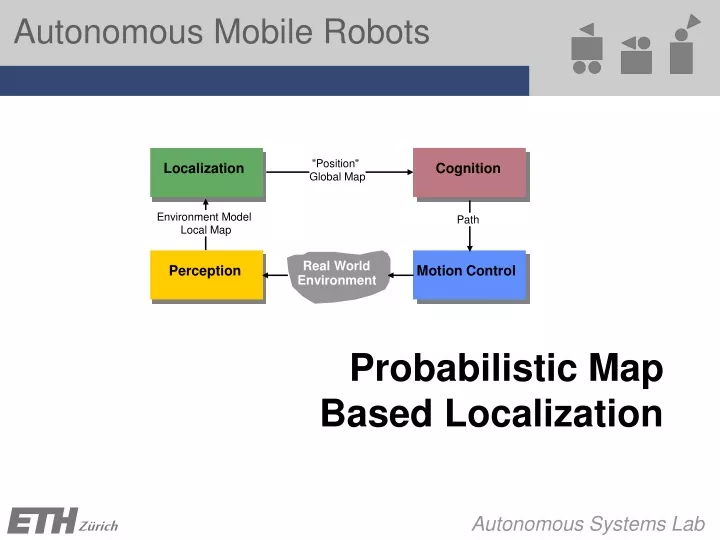
"Position". Localization. Cognition. Global Map. Environment Model. Path. Local Map. Real World. Perception. Motion Control. Environment. Probabilistic Map Based Localization. Outline of today’s lecture. Definition and illustration of probabilistic map based localization

E N D
"Position" Localization Cognition Global Map Environment Model Path Local Map RealWorld Perception Motion Control Environment Probabilistic Map Based Localization
5 - Localization and Mapping Outline of today’s lecture • Definition and illustration of probabilistic map based localization • Two solutions • Markov localization (pages 292-312 of the textbook) • Kalman filter localization (pages 318-338)
5 - Localization and Mapping The problem • Consider a mobile robot moving in a known environment. • As it starts to move, say from a precisely known location, it might keep track of its location using odometry. • However, after a certain movement the robot will get very uncertain about its position => update using an observation of its environment • Observation leads also to an estimate of the robot position which can then be fused with the odometric estimation to get the best possible update of the robots actual position.
5 - Localization and Mapping Illustration of probabilistic bap based localization:Improving belief state by moving The robot is placed somewhere in the environment but it is not told its location The robot queries its sensors and finds it is next to a pillar The robot moves one meter forward. To account for inherent noise in robot motion the new belief is smoother The robot queries its sensors and again it finds itself next to a pillar Finally, it updates its belief by combining this information with its previous belief
5 - Localization and Mapping Why a probabilistic approach for mobile robot localization? • Because the data coming from the robot sensors are affected by measurement errors, we can only compute the probability that the robot is in a given configuration. • The key idea in probabilistic robotics is to represent uncertainty using probability theory: instead of giving a single best estimate of the current robot configuration, probabilistic robotics represents the robot configuration as a probability distribution over the all possible robot poses. This probability is called belief.
Example probability distributions for representing robot configurations • In the following we consider a robot which is constrained to move along a straight rail. The problem is one dimensional. • The robot configuration is the position x along the rail.
5 - Localization and Mapping Example 1: Uniform distribution • This is used when the robot does not know where it is. It means that the information about the robot configuration is null. Remember that in order to be a probability distribution a function p(x) must always satisfy the followingconstraint:
5 - Localization and Mapping Example 2: Multimodal distribution • The robot is in the region around “a” or “b”.
5 - Localization and Mapping Example 3: Dirac distribution • The robot has a probability of 1.0 (i.e. 100%) to be at position “a”. • Note, the Dirac distribution is usually represented with an arrow. • The Dirac function is defined as:
5 - Localization and Mapping Example 4: Gaussian distribution • The Gaussian distribution has the shape of a bell and is defined by the following formula: where μ is the mean value and σ is the standard deviation. • The Gaussian distribution is also called normal distribution and is usually abbreviated with N(μ ,σ ).
5 - Localization and Mapping Description of the probabilistic localization problem • Consider a mobile robot moving in a known environment.
5 - Localization and Mapping Description of the probabilistic localization problem • Consider a mobile robot moving in a known environment. • As it starts to move, say from a precisely known location, it can keep track of its motion using odometry.
5 - Localization and Mapping Description of the probabilistic localization problem • Consider a mobile robot moving in a known environment. • As it starts to move, say from a precisely known location, it can keep track of its motion using odometry. • Due to odometry uncertainty, after some movement the robot will become very uncertain about its position.
5 - Localization and Mapping Description of the probabilistic localization problem • Consider a mobile robot moving in a known environment. • As it starts to move, say from a precisely known location, it can keep track of its motion using odometry. • Due to odometry uncertainty, after some movement the robot will become very uncertain about its position. • To keep position uncertainty from growing unbounded, the robot must localize itself in relation to its environment map. To localize, the robot might use its on-board exteroceptive sensors (e.g. ultrasonic, laser, vision sensors) to make observations of its environment Sensor reference frame
5 - Localization and Mapping Description of the probabilistic localization problem • Consider a mobile robot moving in a known environment. • As it starts to move, say from a precisely known location, it can keep track of its motion using odometry. • Due to odometry uncertainty, after some movement the robot will become very uncertain about its position. • To keep position uncertainty from growing unbounded, the robot must localize itself in relation to its environment map. To localize, the robot might use its on-board exteroceptive sensors (e.g. ultrasonic, laser, vision sensors) to make observations of its environment • The robot updates its position based on the observation. Its uncertainty shrinks. Sensor reference frame
5 - Localization and Mapping Action and perception updates • In robot localization, we distinguish two update steps: • ACTION update: • the robot moves and estimates its position through its proprioceptive sensors. During this step, the robot uncertainty grows. • PERCEPTION update: • the robot makes an observation using its exteroceptive sensors and correct its position by opportunely combining its belief before the observation with the probability of making exactly that observation. During this step, the robot uncertainty shrinks. Probability of making this observation Robot belief before the observation
5 - Localization and Mapping The solution to the probabilistic localization problem Solving the probabilistic localization problem consists in solving separately the Action and Perception updates
5 - Localization and Mapping The solution to the probabilistic localization problem A probabilistic approach to the mobile robot localization problem is a method able to compute the probability distribution of the robot configuration during each Action and Perception step. The ingredients are: • The initial probability distribution • The statistical error model of the proprioceptive sensors (e.g. wheel encoders) • The statistical error model of the exteroceptive sensors (e.g. laser, sonar, camera) • Map of the environment(If the map is not known a priori then the robots needs to build a map of the environment and then localizing in it. This is called SLAM, Simultaneous Localization And Mapping)
5 - Localization and Mapping The solution to the probabilistic localization problem How do we solve the Action and Perception updates? • Action update uses the Theorem of Total probability (or convolution) • Perception update uses the Bayes rule
5 - Localization and Mapping Action update • In this phase the robot estimates its current position based on the knowledge of the previous position and the odometric input • Using the Theorem of Total probability, we compute the robot’s belief after the motion aswhich can be written as a convolution
5 - Localization and Mapping Perception update • In this phase the robot corrects its previous position (i.e. its former belief) by opportunely combining it with the information from its exteroceptive sensors where η is a normalization factor which makes the probability integrate to 1.
5 - Localization and Mapping Perception update • Explanation of This is the probability of observing z given that the robot is at position x, that is:
5 - Localization and Mapping Illustration of probabilistic bap based localization Initial probability distribution Perception update Action update Perception update
5 - Localization and Mapping Illustration of probabilistic bap based localization Initial probability distribution Perception update Action update Perception update
5 - Localization and Mapping Illustration of probabilistic bap based localization Initial probability distribution Perception update Action update Perception update
5 - Localization and Mapping Illustration of probabilistic bap based localization Initial probability distribution Perception update Action update Perception update
5 - Localization and Mapping Markov versus Kalman localization Two approaches exist to represent the probability distribution and to compute the convolution and Bayes rule during the Action and Perception phases
"Position" Localization Cognition Global Map Environment Model Path Local Map RealWorld Perception Motion Control Environment Probabilistic Map Based Localization:Markov LocalizationPages: 292-312 of the textbook
5 - Localization and Mapping Markov localization • Markov localization uses a grid space representation of the robot configuration. • For sake of simplicity let us consider a robot moving in a one dimensional environment (e.g. moving on a rail). Therefore the robot configuration space can be represented through the sole variable x. • Let us discretize the configuration space into 10 cells
5 - Localization and Mapping Markov localization • Let us discretize the configuration space into 10 cells • Suppose that the robot’s initial belief is a uniform distribution from 0 to 3. Observe that all the elements were normalized so that their sum is 1.
5 - Localization and Mapping Markov localization • Initial belief distribution • Action phase: Let us assume that the robot moves forward with the following statistical model • This means that we have 50% probability that the robot moved 2 or 3 cells forward. • Considering what the probability was before moving, what will the probability be after the motion?
5 - Localization and Mapping Markov localization: Action update • The solution is given by the convolution of the two distributions
5 - Localization and Mapping Markov localization: Action update - Explanation • Here, we would like to explain where this formula actually comes from. In order to compute the probability of position x1 in the new belief state, one must sum over all the possible ways in which the robot may reach x1 according to the potential positions expressed in the former belief state x0 and the potential input expressed by u1. Observe that because is limited between 0 and 3, the robot can only reach the states between 2 to 6, therefore • You can now verify that equations that these equations are computing nothing but the convolution of the Action update:
5 - Localization and Mapping Markov localization: Perception update • Let us now assume that the robot uses its onboard range finder and measures the distance from the origin. Assume that the statistical error model of the sensors isThis plot tells us that the distance of the robot from the origin can be equally 5 or 6 units. • What will the final robot belief be after this measurement? The answer is again given by the Bayes rule:
5 - Localization and Mapping Markov Localization: Case Study 2 – Grid Map (5) • Example 2: Museum • Laser scan 1 Courtesy of W. Burgard
5 - Localization and Mapping Markov Localization: Case Study 2 – Grid Map (6) • Example 2: Museum • Laser scan 2 Courtesy of W. Burgard
5 - Localization and Mapping Markov Localization: Case Study 2 – Grid Map (7) • Example 2: Museum • Laser scan 3 Courtesy of W. Burgard
5 - Localization and Mapping Markov Localization: Case Study 2 – Grid Map (8) • Example 2: Museum • Laser scan 13 Courtesy of W. Burgard
5 - Localization and Mapping Markov Localization: Case Study 2 – Grid Map (9) • Example 2: Museum • Laser scan 21 Courtesy of W. Burgard
5 - Localization and Mapping Drawbacks of Markov localization • In the more general planar motion case the grid-map is a three-dimensional array where each cell contains the probability of the robot to be in that cell. In this case, the cell size must be chosen carefully. • During each prediction and measurement steps, all the cells are updated. If the number of cells in the map is too large, the computation can become too heavy for real-time operations. • The convolution in a 3D space is clearly the computationally most expensive step. • As an example, consider a 30x30 m environment and a cell size of 0.1 m x 0.1 m x 1 deg. In this case, the number of cells which need to be updated at each step would be 30x30x100x360=32.4 million cells!Fine fixed decomposition grids result in a huge state space • Very important processing power needed • Large memory requirement
5 - Localization and Mapping Drawbacks of Markov localization • Reducing complexity • Various approached have been proposed for reducing complexity • One possible solution would be to increase the cell size at the expense of localization accuracy. • Another solution is to use an adaptive cell decomposition instead of a fixed cell decomposition. • Randomized Sampling / Particle Filter • The main goal is to reduce the number of states that are updated in each step • Approximated belief state by representing only a ‘representative’ subset of all states (possible locations) • E.g update only 10% of all possible locations • The sampling process is typically weighted, e.g. put more samples around the local peaks in the probability density function • However, you have to ensure some less likely locations are still tracked, otherwise the robot might get lost