Download
1 / 44
440 likes | 562 Views
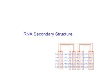
RNA Secondary Structure. aagacuucggaucuggcgacaccc uacacuucggaugacaccaaagug aggucuucggcacgggcaccauuc ccaacuucggauuuugcuaccaua aagccuucggagcgggcguaacuc. Decoding: the CYK algorithm. Given x = x 1 ....x N , and a SCFG G, Find the most likely parse of x

E N D
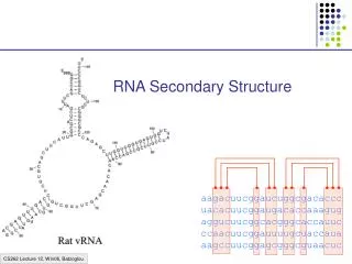
RNA Secondary Structure aagacuucggaucuggcgacaccc uacacuucggaugacaccaaagug aggucuucggcacgggcaccauuc ccaacuucggauuuugcuaccaua aagccuucggagcgggcguaacuc
Decoding: the CYK algorithm Given x = x1....xN, and a SCFG G, Find the most likely parse of x (the most likely alignment of G to x) Dynamic programming variable: (i, j, V): likelihood of the most likely parse of xi…xj, rooted at nonterminal V Then, (1, N, S): likelihood of the most likely parse of x by the grammar
V X Y j i The CYK algorithm (Cocke-Younger-Kasami) Initialization: For i = 1 to N, any nonterminal V, (i, i, V) = log P(V xi) Iteration: For i = 1 to N – 1 For j = i+1 to N For any nonterminal V, (i, j, V) = maxXmaxYmaxik<j (i,k,X) + (k+1,j,Y) + log P(VXY) Termination: log P(x | , *) = (1, N, S) Where * is the optimal parse tree (if traced back appropriately from above)
A SCFG for predicting RNA structure S a S | c S | g S | u S | S a | S c | S g | S u a S u | c S g | g S u | u S g | g S c | u S a SS • Adjust the probability parameters to reflect bond strength etc • No distinction between non-paired bases, bulges, loops • Can modify to model these events • L: loop nonterminal • H: hairpin nonterminal • B: bulge nonterminal • etc
CYK for RNA folding Initialization: (i, i-1) = log P() Iteration: For i = 1 to N For j = i to N (i+1, j–1) + log P(xi S xj) (i, j–1) + log P(S xi) (i, j) = max (i+1, j) + log P(xi S) maxi < k < j (i, k) + (k+1, j) + log P(S S)
Evaluation Recall HMMs: Forward: fl(i) = P(x1…xi, i = l) Backward: bk(i) = P(xi+1…xN | i = k) Then, P(x) = k fk(N) ak0 = l a0l el(x1) bl(1) Analogue in SCFGs: Inside: a(i, j, V) = P(xi…xj is generated by nonterminal V) Outside: b(i, j, V) = P(x, excluding xi…xj is generated by S and the excluded part is rooted at V)
The Inside Algorithm To compute a(i, j, V) = P(xi…xj, produced by V) a(i, j, v) = X Y k a(i, k, X) a(k+1, j, Y) P(V XY) V X Y j i k k+1
Algorithm: Inside Initialization: For i = 1 to N, V a nonterminal, a(i, i, V) = P(V xi) Iteration: For i = 1 to N-1 For j = i+1 to N For V a nonterminal a(i, j, V) = X Y k a(i, k, X) a(k+1, j, X) P(V XY) Termination: P(x | ) = a(1, N, S)
The Outside Algorithm b(i, j, V) = Prob(x1…xi-1, xj+1…xN, where the “gap” is rooted at V) Given that V is the right-hand-side nonterminal of a production, b(i, j, V) = X Y k<i a(k, i – 1, X) b(k, j, Y) P(Y XV) Y V X j i k
Algorithm: Outside Initialization: b(1, N, S) = 1 For any other V, b(1, N, V) = 0 Iteration: For i = 1 to N-1 For j = N down to i For V a nonterminal b(i, j, V) = X Y k<i a(k, i – 1, X) b(k, j, Y) P(Y XV) + X Y k<i a(j+1, k, X) b(i, k, Y) P(Y VX) Termination: It is true for any i, that: P(x | ) = X b(i, i, X) P(X xi)
Learning for SCFGs We can now estimate c(V) = expected number of times V is used in the parse of x1….xN 1 c(V) = –––––––– 1iNijN a(i, j, V) b(i, j, v) P(x | ) 1 c(VXY) = –––––––– 1iNi<jN ik<j b(i,j,V) a(i,k,X) a(k+1,j,Y) P(VXY) P(x | )
Learning for SCFGs Then, we can re-estimate the parameters with EM, by: c(VXY) Pnew(VXY) = –––––––––––– c(V) c(V a) i: xi = a b(i, i, V) P(V a) Pnew(V a) = –––––––––– = –––––––––––––––––––––––––––––––– c(V) 1iNi<jN a(i, j, V) b(i, j, V)
Summary: SCFG and HMM algorithms GOALHMM algorithm SCFG algorithm Optimal parse Viterbi CYK Estimation Forward Inside Backward Outside Learning EM: Fw/Bck EM: Ins/Outs Memory Complexity O(N K) O(N2 K) Time Complexity O(N K2) O(N3 K3) Where K: # of states in the HMM # of nonterminals in the SCFG
position i length l 5’ 5’ position i 3’ 3’ position j position j The Zuker algorithm – main ideas Models energy of a fold in terms of specific features: • Pairs of base pairs (stacked pairs) • Bulges • Loops (size, composition) • Interactions between stem and loop position j’ positions i 5’ position j 3’
1 4 3 5 2 5 2 3 1 4 Phylogeny Tree Reconstruction
Inferring Phylogenies Trees can be inferred by several criteria: • Morphology of the organisms • Can lead to mistakes! • Sequence comparison Example: Orc: ACAGTGACGCCCCAAACGT Elf: ACAGTGACGCTACAAACGT Dwarf: CCTGTGACGTAACAAACGA Hobbit: CCTGTGACGTAGCAAACGA Human: CCTGTGACGTAGCAAACGA
Modeling Evolution During infinitesimal time t, there is not enough time for two substitutions to happen on the same nucleotide So we can estimate P(x | y, t), for x, y {A, C, G, T} Then let P(A|A, t) …… P(A|T, t) S(t) = … … … … P(T|A, t) …… P(T|T, t) x x t y
Modeling Evolution A C Reasonable assumption: multiplicative (implying a stationary Markov process) S(t+t’) = S(t)S(t’) That is, P(x | y, t+t’) = z P(x | z, t) P(z | y, t’) Jukes-Cantor: constant rate of evolution 1 - 3 For short time , S() = I+R = 1 - 3 1 - 3 1 - 3 T G
Modeling Evolution Jukes-Cantor: For longer times, r(t) s(t) s(t) s(t) S(t) = s(t) r(t) s(t) s(t) s(t) s(t) r(t) s(t) s(t) s(t) s(t) r(t) Where we can derive: r(t) = ¼ (1 + 3 e-4t) s(t) = ¼ (1 – e-4t) S(t+) = S(t)S() = S(t)(I + R) Therefore, (S(t+) – S(t))/ = S(t) R At the limit of 0, S’(t) = S(t) R Equivalently, r’ = -3r + 3s s’ = -s + r Those diff. equations lead to: r(t) = ¼ (1 + 3 e-4t) s(t) = ¼ (1 – e-4t)
Modeling Evolution Kimura: Transitions: A/G, C/T Transversions: A/T, A/C, G/T, C/G Transitions (rate ) are much more likely than transversions (rate ) r(t)s(t)u(t)s(t) S(t) = s(t)r(t)s(t)u(t) u(t)s(t)r(t)s(t) s(t)u(t)s(t)r(t) Where s(t) = ¼ (1 – e-4t) u(t) = ¼ (1 + e-4t – e-2(+)t) r(t) = 1 – 2s(t) – u(t)
Phylogeny and sequence comparison Basic principles: • Degree of sequence difference is proportional to length of independent sequence evolution • Only use positions where alignment is pretty certain – avoid areas with (too many) gaps
Distance between two sequences Given sequences xi, xj, Define dij = distance between the two sequences One possible definition: dij = fraction f of sites u where xi[u] xj[u] Better model (Jukes-Cantor): f = 3 s(t) = ¾ (1 – e-4t) ¾ e-4t = ¾ – f log (e-4t) = log (1 – 4/3 f) -4t = log(1 – 4/3 f) dij = t = - ¼ -1 log(1 – 4/3 f)
A simple clustering method for building tree UPGMA (unweighted pair group method using arithmetic averages) Or the Average Linkage Method Given two disjoint clusters Ci, Cj of sequences, 1 dij = ––––––––– {p Ci, q Cj}dpq |Ci| |Cj| Claim that if Ck = Ci Cj, then distance to another cluster Cl is: dil |Ci| + djl |Cj| dkl = –––––––––––––– |Ci| + |Cj| Proof Ci,Cl dpq + Cj,Cl dpq dkl = –––––––––––––––– (|Ci| + |Cj|) |Cl| |Ci|/(|Ci||Cl|) Ci,Cl dpq + |Cj|/(|Cj||Cl|) Cj,Cl dpq = –––––––––––––––––––––––––––––––––––– (|Ci| + |Cj|) |Ci| dil + |Cj| djl = ––––––––––––– (|Ci| + |Cj|)
Algorithm: Average Linkage 1 4 Initialization: Assign each xi into its own cluster Ci Define one leaf per sequence, height 0 Iteration: Find two clusters Ci, Cj s.t. dij is min Let Ck = Ci Cj Define node connecting Ci, Cj, & place it at height dij/2 Delete Ci, Cj Termination: When two clusters i, j remain, place root at height dij/2 3 5 2 5 2 3 1 4
Example 4 3 2 1 v w x y z
Ultrametric Distances and Molecular Clock Definition: A distance function d(.,.) is ultrametric if for any three distances dij dik dij, it is true that dij dik = dij The Molecular Clock: The evolutionary distance between species x and y is 2 the Earth time to reach the nearest common ancestor That is, the molecular clock has constant rate in all species The molecular clock results in ultrametric distances years 1 4 2 3 5
Ultrametric Distances & Average Linkage Average Linkage is guaranteed to reconstruct correctly a binary tree with ultrametric distances Proof: Exercise 5 1 4 2 3
Weakness of Average Linkage Molecular clock: all species evolve at the same rate (Earth time) However, certain species (e.g., mouse, rat) evolve much faster Example where UPGMA messes up: AL tree Correct tree 3 2 1 3 4 4 2 1
d1,4 Additive Distances 1 Given a tree, a distance measure is additive if the distance between any pair of leaves is the sum of lengths of edges connecting them Given a tree T & additive distances dij, can uniquely reconstruct edge lengths: • Find two neighboring leaves i, j, with common parent k • Place parent node k at distance dkm = ½ (dim + djm – dij) from any node m 4 12 8 3 13 7 9 5 11 10 6 2
Reconstructing Additive Distances Given T x T D y 5 4 3 z 3 4 w 7 6 v If we know T and D, but do not know the length of each leaf, we can reconstruct those lengths
Reconstructing Additive Distances Given T x T D y z w v
Reconstructing Additive Distances Given T D x T y z a w D1 v dax = ½ (dvx + dwx – dvw) day = ½ (dvy + dwy – dvw) daz = ½ (dvz + dwz – dvw)
Reconstructing Additive Distances Given T D1 x T y 5 4 b 3 z 3 a 4 c w 7 D2 6 d(a, c) = 3 d(b, c) = d(a, b) – d(a, c) = 3 d(c, z) = d(a, z) – d(a, c) = 7 d(b, x) = d(a, x) – d(a, b) = 5 d(b, y) = d(a, y) – d(a, b) = 4 d(a, w) = d(z, w) – d(a, z) = 4 d(a, v) = d(z, v) – d(a, z) = 6 Correct!!! v D3
Neighbor-Joining • Guaranteed to produce the correct tree if distance is additive • May produce a good tree even when distance is not additive Step 1: Finding neighboring leaves Define Dij = dij – (ri + rj) Where 1 ri = –––––k dik |L| - 2 Claim: The above “magic trick” ensures that Dij is minimal iffi, j are neighbors Proof: Very technical, please read Durbin et al.! 1 3 0.1 0.1 0.1 0.4 0.4 4 2
Algorithm: Neighbor-joining Initialization: Define T to be the set of leaf nodes, one per sequence Let L = T Iteration: Pick i, j s.t. Dij is minimal Define a new node k, and set dkm = ½ (dim + djm – dij) for all m L Add k to T, with edges of lengths dik = ½ (dij + ri – rj) Remove i, j from L; Add k to L Termination: When L consists of two nodes, i, j, and the edge between them of length dij
Parsimony – What if we don’t have distances • One of the most popular methods: • GIVEN multiple alignment • FIND tree & history of substitutions explaining alignment Idea: Find the tree that explains the observed sequences with a minimal number of substitutions Two computational subproblems: • Find the parsimony cost of a given tree (easy) • Search through all tree topologies (hard)
Example {A} Final cost C = 1 {A} {A, B} Cost C+=1 A A B A {B} {A} {A} {A}
Parsimony Scoring Given a tree, and an alignment column u Label internal nodes to minimize the number of required substitutions Initialization: Set cost C = 0; k = 2N – 1 Iteration: If k is a leaf, set Rk = { xk[u] } If k is not a leaf, Let i, j be the daughter nodes; Set Rk = Ri Rj if intersection is nonempty Set Rk = Ri Rj, and C += 1, if intersection is empty Termination: Minimal cost of tree for column u, = C
Example {B} {A,B} {A} {B} {A} {A,B} {A} A A A A B B A B {A} {A} {A} {A} {B} {B} {A} {B}
Probabilistic Methods A more refined measure of evolution along a tree than parsimony P(x1, x2, xroot | t1, t2) = P(xroot) P(x1 | t1, xroot) P(x2 | t2, xroot) If we use Jukes-Cantor, for example, and x1 = xroot = A, x2 = C, t1 = t2 = 1, = pA¼(1 + 3e-4α) ¼(1 – e-4α) = (¼)3(1 + 3e-4α)(1 – e-4α) xroot t1 t2 x1 x2
Probabilistic Methods xroot • If we know all internal labels xu, P(x1, x2, …, xN, xN+1, …, x2N-1 | T, t) = P(xroot)jrootP(xj | xparent(j), tj, parent(j)) • Usually we don’t know the internal labels, therefore P(x1, x2, …, xN | T, t) = xN+1 xN+2 … x2N-1P(x1, x2, …, x2N-1 | T, t) xu x2 xN x1
Felsenstein’s Likelihood Algorithm Let P(Lk | a) denote the prob. of all the leaves below node k, given that the residue at k is a To calculate P(x1, x2, …, xN | T, t) Initialization: Set k = 2N – 1 Iteration: Compute P(Lk | a) for all a If k is a leaf node: Set P(Lk | a) = 1(a = xk) If k is not a leaf node: 1. Compute P(Li | b), P(Lj | b) for all b, for daughter nodes i, j 2. Set P(Lk | a) = b,c P(b | a, ti) P(Li | b) P(c | a, tj) P(Lj | c) Termination: Likelihood at this column = P(x1, x2, …, xN | T, t) = aP(L2N-1 | a)P(a)
Probabilistic Methods Given M (ungapped) alignment columns of N sequences, • Define likelihood of a tree: L(T, t) = P(Data | T, t) = m=1…M P(x1m, …, xnm, T, t) Maximum Likelihood Reconstruction: • Given data X = (xij), find a topology T and length vector t that maximize likelihood L(T, t)
Current popular methods HUNDREDS of programs available! http://evolution.genetics.washington.edu/phylip/software.html#methods Some recommended programs: • Discrete—Parsimony-based • Rec-1-DCM3 http://www.cs.utexas.edu/users/tandy/mp.html Tandy Warnow and colleagues • Probabilistic • SEMPHY http://www.cs.huji.ac.il/labs/compbio/semphy/ Nir Friedman and colleagues