K-means and Kohonen Maps Unsupervised Clustering Techniques

1. K-means and Kohonen MapsUnsupervised Clustering Techniques Steve Hookway 4/8/04

2. What is a DNA Microarray? • An experiment on the order of 10k elements • A way to explore the function of a gene • A snapshot of the expression level of an entire phenotype under given test conditions

3. Some Microarray Terminology • Probe: ssDNA printed on the solid substrate (nylon or glass) These are the genes we are going to be testing • Target: cDNA which has been labeled and is to be washed over the probe

4. Microarray Fabrication • Deposition of DNA fragments • Deposition of PCR-amplified cDNA clones • Printing of already synthesized oligonucleotieds • In Situ synthesis • Photolithography • Ink Jet Printing • Electrochemical Synthesis From “Data Analysis Tools for DNA Microarrays” by Sorin Draghici

5. cDNA Microarrays and Oligonucleotide Probes From “Data Analysis Tools for DNA Microarrays” by Sorin Draghici

6. In Situ Synthesis • Photochemically synthesized on the chip • Reduces noise caused by PCR, cloning, and Spotting • As previously mentioned, three kinds of In Situ Synthesis • Photolithography • Ink Jet Printing • Electrochemical Synthesis From “Data Analysis Tools for DNA Microarrays” by Sorin Draghici

7. Photolithography Photodeprotection • Similar to process used to build VLSI circuits • Photolithographic masks are used to add each base • If base is present, there will be a hole in the corresponding mask • Can create high density arrays, but sequence length is limited mask C From “Data Analysis Tools for DNA Microarrays” by Sorin Draghici

8. Ink Jet Printing • Four cartridges are loaded with the four nucleotides: A, G, C,T • As the printer head moves across the array, the nucleotides are deposited where they are needed From “Data Analysis Tools for DNA Microarrays” by Sorin Draghici

9. Electrochemical Synthesis • Electrodes are embedded in the substrate to manage individual reaction sites • Electrodes are activated in necessary positions in a predetermined sequence that allows the sequences to be constructed base by base • Solutions containing specific bases are washed over the substrate while the electrodes are activated From “Data Analysis Tools for DNA Microarrays” by Sorin Draghici

10. http://www.bio.davidson.edu/courses/genomics/chip/chip.html

11. Application of Microarrays • We only know the function of about 20% of the 30,000 genes in the Human Genome • Gene exploration • Faster and better • Can be used for DNA computing http://www.gene-chips.com/sample1.html From “Data Analysis Tools for DNA Microarrays” by Sorin Draghici

12. A Data Mining Problem • On a given Microarray we test on the order of 10k elements at a time • Data is obtained faster than it can be processed • We need some ways to work through this large data set and make sense of the data

13. Grouping and Reduction • Grouping: discovers patterns in the data from a microarray • Reduction: reduces the complexity of data by removing redundant probes (genes) that will be used in subsequent assays

14. Unsupervised Grouping: Clustering • Pattern discovery via grouping similarly expressed genes together • Three techniques most often used • k-Means Clustering • Hierarchical Clustering • Kohonen Self Organizing Feature Maps

15. Clustering Limitations • Any data can be clustered, therefore we must be careful what conclusions we draw from our results • Clustering is non-deterministic and can and will produce different results on different runs

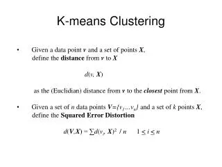
16. K-means Clustering • Given a set of n data points in d-dimensional space and an integer k • We want to find the set of k points in d-dimensional space that minimizes the mean squared distance from each data point to its nearest center • No exact polynomial-time algorithms are known for this problem “A Local Search Approximation Algorithm for k-Means Clustering” by Kanungo et. al

17. K-means Algorithm (Lloyd’s Algorithm) • Has been shown to converge to a locally optimal solution • But can converge to a solution arbitrarily bad compared to the optimal solution Data Points Optimal Centers Heuristic Centers K=3 • “K-means-type algorithms: A generalized convergence theorem and characterization of local optimality” by Selim and Ismail • “A Local Search Approximation Algorithm for k-Means Clustering” by Kanungo et al.

18. Euclidean Distance Now to find the distance between two points, say the origin and the point (3,4): Simple and Fast! Remember this when we consider the complexity!

19. Finding a Centroid We use the following equation to find the n dimensional centroid point amid k n dimensional points: Let’s find the midpoint between 3 2D points, say: (2,4) (5,2) (8,9)

20. K-means Algorithm • Choose k initial center points randomly • Cluster data using Euclidean distance (or other distance metric) • Calculate new center points for each cluster using only points within the cluster • Re-Cluster all data using the new center points • This step could cause data points to be placed in a different cluster • Repeat steps 3 & 4 until the center points have moved such that in step 4 no data points are moved from one cluster to another or some other convergence criteria is met From “Data Analysis Tools for DNA Microarrays” by Sorin Draghici

21. An example with k=2 • We Pick k=2 centers at random • We cluster our data around these center points Figure Reproduced From “Data Analysis Tools for DNA Microarrays” by Sorin Draghici

22. K-means example with k=2 • We recalculate centers based on our current clusters Figure Reproduced From “Data Analysis Tools for DNA Microarrays” by Sorin Draghici

23. K-means example with k=2 • We re-cluster our data around our new center points Figure Reproduced From “Data Analysis Tools for DNA Microarrays” by Sorin Draghici

24. K-means example with k=2 We repeat the last two steps until no more data points are moved into a different cluster Figure Reproduced From “Data Analysis Tools for DNA Microarrays” by Sorin Draghici

25. Choosing k • Use another clustering method • Run algorithm on data with several different values of k • Use advance knowledge about the characteristics of your test • Cancerous vs Non-Cancerous

26. Cluster Quality • Since any data can be clustered, how do we know our clusters are meaningful? • The size (diameter) of the cluster vs. The inter-cluster distance • Distance between the members of a cluster and the cluster’s center • Diameter of the smallest sphere From “Data Analysis Tools for DNA Microarrays” by Sorin Draghici

27. Cluster Quality Continued distance=5 size=5 distance=20 Quality of cluster assessed by ratio of distance to nearest cluster and cluster diameter size=5 Figure Reproduced From “Data Analysis Tools for DNA Microarrays” by Sorin Draghici

28. Cluster Quality Continued Quality can be assessed simply by looking at the diameter of a cluster A cluster can be formed even when there is no similarity between clustered patterns. This occurs because the algorithm forces k clusters to be created. From “Data Analysis Tools for DNA Microarrays” by Sorin Draghici

29. Characteristics of k-means Clustering • The random selection of initial center points creates the following properties • Non-Determinism • May produce clusters without patterns • One solution is to choose the centers randomly from existing patterns From “Data Analysis Tools for DNA Microarrays” by Sorin Draghici

30. Algorithm Complexity • Linear in the number of data points, N • Can be shown to have time of cN • c does not depend on N, but rather the number of clusters, k • Low computational complexity • High speed From “Data Analysis Tools for DNA Microarrays” by Sorin Draghici

31. The Need for a New Algorithm • Each data point is assigned to the correct cluster • Data points that seem to be far away from each other in heuristic are in reality very closely related to each other Figure Reproduced From “Data Analysis Tools for DNA Microarrays” by Sorin Draghici

32. The Need for a New Algorithm Eisen et al., 1998

33. Kohonen Self Organizing Feature Maps (SOFM) • Creates a map in which similar patterns are plotted next to each other • Data visualization technique that reduces n dimensions and displays similarities • More complex than k-means or hierarchical clustering, but more meaningful • Neural Network Technique • Inspired by the brain From “Data Analysis Tools for DNA Microarrays” by Sorin Draghici

34. SOFM Description • Each unit of the SOFM has a weighted connection to all inputs • As the algorithm progresses, neighboring units are grouped by similarity Output Layer Input Layer From “Data Analysis Tools for DNA Microarrays” by Sorin Draghici

35. SOFM Algorithm Initialize Map For t from 0 to 1 //t is the learning factor Randomly select a sample Get best matching unit Scale neighbors Increase t a small amount //decrease learning factor End for From: http://davis.wpi.edu/~matt/courses/soms/

36. An Example Using Color Three dimensional data: red, blue, green Will be converted into 2D image map with clustering of Dark Blue and Greys together and Yellow close to Both the Red and the Green From http://davis.wpi.edu/~matt/courses/soms/

37. An Example Using Color Each color in the map is associated with a weight From http://davis.wpi.edu/~matt/courses/soms/

38. An Example Using Color • Initialize the weights Random Values Colors in the Corners Equidistant From http://davis.wpi.edu/~matt/courses/soms/

39. An Example Using Color Continued • Get best matching unit After randomly selecting a sample, go through all weight vectors and calculate the best match (in this case using Euclidian distance) Think of colors as 3D points each component (red, green, blue) on an axis From http://davis.wpi.edu/~matt/courses/soms/

40. An Example Using Color Continued • Getting the best matching unit continued… For example, lets say we chose green as the sample. Then it can be shown that light green is closer to green than red: Green: (0,6,0) Light Green: (3,6,3) Red(6,0,0) This step is repeated for entire map, and the weight with the shortest distance is chosen as the best match From http://davis.wpi.edu/~matt/courses/soms/

41. An Example Using Color Continued • Scale neighbors • Determine which weights are considred nieghbors • How much each weight can become more like the sample vector • Determine which weights are considered neighbors • In the example, a gaussian function is used where every point above 0 is considered a neighbor From http://davis.wpi.edu/~matt/courses/soms/

42. An Example Using Color Continued • How much each weight can become more like the sample When the weight with the smallest distance is chosen and the neighbors are determined, it and its neighbors ‘learn’ by changing to become more like the sample…The farther away a neighbor is, the less it learns From http://davis.wpi.edu/~matt/courses/soms/

43. An Example Using Color Continued NewColorValue = CurrentColor*(1-t)+sampleVector*t For the first iteration t=1 since t can range from 0 to 1, for following iterations the value of t used in this formula decreases because there are fewer values in the range (as t increases in the for loop) From http://davis.wpi.edu/~matt/courses/soms/

44. Conclusion of Example Samples continue to be chosen at random until t becomes 1 (learning stops) At the conclusion of the algorithm, we have a nicely clustered data set. Also note that we have achieved our goal: Similar colors are grouped closely together From http://davis.wpi.edu/~matt/courses/soms/

45. SOFM Applied to Genetics • Consider clustering 10,000 genes • Each gene was measured in 4 experiments • Input vectors are 4 dimensional • Initial pattern of 10,000 each described by a 4D vector • Each of the 10,000 genes is chosen one at a time to train the SOM From “Data Analysis Tools for DNA Microarrays” by Sorin Draghici

46. SOFM Applied to Genetics • The pattern found to be closest to the current gene (determined by weight vectors) is selected as the winner • The weight is then modified to become more similar to the current gene based on the learning rate (t in the previous example) • The winner then pulls its neighbors closer to the current gene by causing a lesser change in weight From “Data Analysis Tools for DNA Microarrays” by Sorin Draghici

47. SOFM Applied to Genetics • This process continues for all 10,000 genes • Process is repeated until over time the learning rate is reduced to zero From “Data Analysis Tools for DNA Microarrays” by Sorin Draghici

48. Our Favorite Example With Yeast • Reduce data set to 828 genes • Clustered data into 30 clusters using a SOFM • Each pattern is represented by its average (centroid) pattern • Clustered data has same behavior • Neighbors exhibit similar behavior “Interpresting patterns of gene expression with self-organizing maps: Methods and application to hematopoietic differentiation” by Tamayo et al.

49. A SOFM Example With Yeast “Interpresting patterns of gene expression with self-organizing maps: Methods and application to hematopoietic differentiation” by Tamayo et al.

50. Benefits of SOFM • SOFM contains the set of features extracted from the input patterns (reduces dimensions) • SOFM yields a set of clusters • A gene will always be most similar to a gene in its immediate neighborhood than a gene further away From “Data Analysis Tools for DNA Microarrays” by Sorin Draghici