Download
1 / 12
130 likes | 223 Views
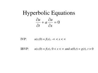
Hyperbolic Equations. Pure IVP:. Lax-Wendroff method. Preliminaries: Input: Integer p, lower spatial index at t jmax Integer q, upper spatial index at t jmax Integer jmax, number of time steps real k, time step real h, space step real a, coefficient

E N D
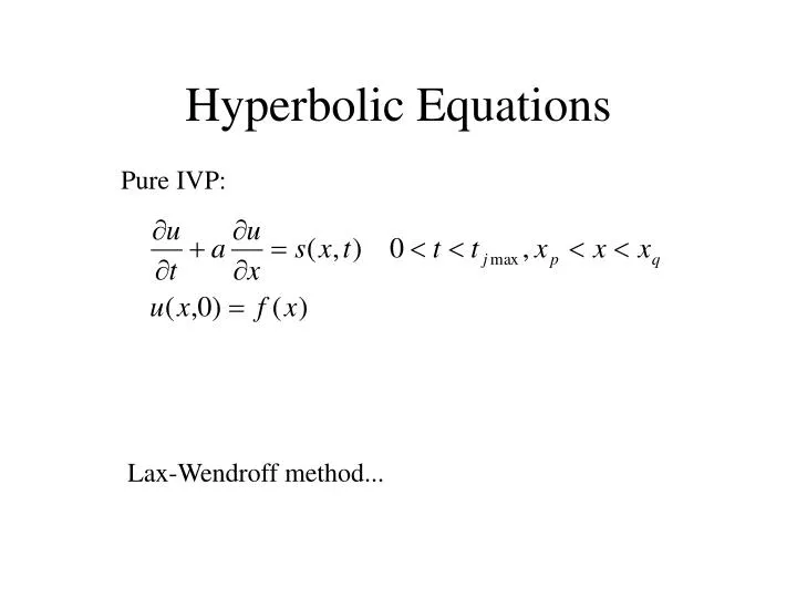
Hyperbolic Equations Pure IVP: Lax-Wendroff method...
Preliminaries: Input: Integer p, lower spatial index at tjmax Integer q, upper spatial index at tjmax Integer jmax, number of time steps real k, time step real h, space step real a, coefficient function f(x), initial condition function ss(x,t), source term functions (sx(x,t) and st(x,t), respectively)
Define Grid: s = k/h check stability Initialize (outputting initial condition) t = 0 nmin = p – jmax nmax = q + jmax for n = nmin, nmin+1, …, nmax xn = n*h V(n) = f(xn) endloop output t for n = p, p+1, …, q output V(n) endloop
Time Loop: for j = 1, 2, …, jmax nmin = nmin+1 nmax = nmax-1 for n = nmin, nmin+1, …, nmax U(n) = V(n)-0.5*s*a*(V(n+1)-V(n-1)) + s**2*a**2/2*(V(n-1)-2*V(n)+V(n+1) + k*ss(n*h,t)+k**2/2*(st(n*h,t)-a*sx(n*h,t)) endloop t = t + k for n = nmin, nmin+1, …, nmax V(n) = U(n) endloop output t for n = p, p+1, …, q output V(n) endloop endloop
Wendroff implicit method for the IBVP Preliminaries: Input: Integer nmax, maximum x index Integer jmax, number of time steps real k, time step real h, space step real a, coefficient function f(x), initial condition function g(t), boundary condition function ss(x,t), source term
Define Grid: s = k/h Initialize (outputting initial condition) t = 0 xmax = nmax*h for n = 0, 1, …, nmax xn = n*h V(n) = f(xn) endloop output t for n = p, p+1, …, q output V(n) endloop
Time Loop: • for j = 1, 2, …, jmax • t = t + k • U(0) = g(t) • q = (1-s*a)/(1+s*a) • for n = 0, 1, …, nmax-1 • U(n+1) = V(n)+q*V(n+1)-q*U(n) • +2*k*ss(xmax+h/2, t-k/2)/(1+s*a) • endloop • for n = 0, 1, …, nmax • V(n) = U(n) • endloop • output t • for n = 0, 1, …, nmax • output U(n) • endloop • endloop
The Wendroff method (among others) does not require specification of a downstream boundary condition, but others, like the Lax-Wendroff do. This can be done either numerically or with some physical reasoning. Numerical: characteristics (skip) finite difference approximation Issues: stability and accuracy
Conservation Law Form recall...
Conservation Law Form Conservation law form if FD equation can be cast as: where Q is a numerical approximation of the flux at “cell” boundaries:
Conservation Law Form write eqn. as: Lax-Friedrichs method where