Download
1 / 54
550 likes | 771 Views
An introduction to PFLOTRAN and its application to CO 2 geological storage problems Edinburgh, 10 January 2014 Paolo Orsini. PFLOTRAN overview

E N D
An introduction to PFLOTRAN and its application to CO2 geological storage problems Edinburgh, 10 January 2014 Paolo Orsini
PFLOTRAN overview Parallel n-phases n-components reactive flow code for modeling sub-surface processes, developed by the cooperation of four US national labs (LANL, PNNL, ORNL, LBNL): Open Source GNU Lesser General Public License (LGPL) Object oriented programming (F95, F2003-2008): easy to extend and to incorporate additional processes Parallel computation based on the PETSC library (ANL lab) Parallel implementation tested on computer architectures with >100k processor cores
PFLOTRAN modeling capabilities Solution of mass balance and energy equations that can be coupled sequentially to reactive-transport and quasi-static geo-mechanical models: Single phase variable saturated flow (Richards equation) TH (Thermal Hydrologic) Single phase variable saturated flow with variable density (function of p and T) Immiscible CO2 – brine: non-isothermal two-phase flow Supercritical CO2 – brine: non-isothermal two-phase two-components flow (Variable switch) Development of a black oil model (FVFs) is at planning stage
Variable saturated flow problems • 270 M DOF • Time[s]: wall clock time per time step Example of parallel performance on a super computer: Richards Equation (Hanford 300 Area)
CO2-Brine: 25 M cells • Yellowstone machine: 8000 cores • Flow: 3 DOF • Transport: 10 DOF • Time[s] for 10 flow step + 14 transport steps Example of parallel performance on a super computer: CO2-Brine
PETSc (Portable extensible toolkit for scientific computing) parallel framework - overview Data structure for a parallel (CSR matrices, Blocked CSR matrices, distributed arrays, etc) Non linear solvers (Newton-based methods) Pre-conditioners ( Additive Swartz, ILU, etc..) Time stepper algorithms (Euler, Backward Euler, etc) Krylov Subspace methods (GMRES, CG, CGS, etc)
Discretisation Space: Control volume (structured and unstructured grids), two point flux formula, MFD under development Time: Flow solvers: implicit Reactive transport Fully implicit Operator splitting (require less memory but also to satisfy the CFL condition for stability Coupling Sequential between flow and reactive transport
Domain decomposition Parallelisation based on overlapping-domain decomposition (each processor is assigned to a sub-domain): accumulation terms are easy to compute because are local operations, computation of fluxes require message passing
Domain decomposition To evaluate a local function f(x), each process requires the local portion of x and its ghosted part (overlapping part)
General n-phase n-components mass balance and energy equations Mass balance equation Energy equation • sαphase saturation, η molar density,Xiαmolar fraction of componentiin phaseα, Dαphase diffusivity coefficient, φporosity, Henthalpy, Uinternal energy, ρrrock density, κthermal diffusivity coefficient, kαrelative permeability,ksaturated media permeability
General n-phase n-components mass balance and energy equations: degrees of freedom Gibbs phase rule Open System Unknowns Constraints Degrees of freedom (Ndof)
MPHASE - CO2-Brine module: governing equations Two phase [gas, liquid], two components [CO2, H2O]: 3 DOF Two component mass balance:
MPHASE – CO2-Brine module: auxiliary variables The pure CO2 properties, which depend on P and T, are computed with the Spang & Wagner (1994) EOS. They are tabulated before the computation, and a look-up table is used during the simulation Brine/CO2 mixture density Duan (2008): Solubility of CO2 in brine, Duan and Sun (2003): Solution procedure by variable switch approach
MPHASE CO2-Brine Module: pressure and temperature range limits The code standard release is limited to Supercritical CO2, however the real limit is the number of phases (CO2 liquid and gas cannot coexist)
Geomechanics Model Governing equations (quasi-static equilibrium) • λ and μ are the Lame parameters, related to the Young’s modulus and Poisson ratio.α= coefficient of thermal expansionβ=Biot’s coefficient
Equation is solved with the Galerkin finite element method. • One-way coupling with the flow solver via pressure and temperature, which are available at the control volume cell centres. • The geo-mechanics does not need to be solved at every flow time step. • The cell centres are the nodes of the finite element mesh, so there is no need of interpolating P and T. (Voronoi mesh) Geomechanics model – Discretisation • CV mesh for flow solution • FEM mesh geomechanics
PFLOTRAN – Pre-Post processors There is no specific pre-processor Geological model and grid generation with external software Several mesh formats: (i) structured with variable spacing [internal generator], (ii) implicit unstructured [list of nodes and connectivity table for hex, wedges, pyramids and tets], (iii) explicit unstructured [list of cell centre volumes and connecting faces, for general polyhedrons] Simulation control parameters, BCs and ICs via flexible text files Post-processor Open source, VisIt, ParaView. Both can post-process remotely, on parallel architectures (auto-reassembling). Commercial software: Tecplot
Input deck file to set up the simulation control parametres – organised in cards Grid (internal mesh generator or external mesh) Specify flow mode (the application module: e.g. CO2-brine, Richards) Material properties Capillary & relative permeability functions Regions: interior domain and surfaces Geometry may be specified independent of grid Initial & boundary conditions, source/sinks for flow and transport Coupler: to couple regions with initial and boundary conditions Solvers (direct, Iterative) Time stepping Output Checkpoint/Restart
Input deck file example: grid, regions, material, strata Each card containing multiple instructions starts by its key word and ends by “END” or “/”
Input deck file example: flow conditions & initial and boundary condition couplers A line of the input deck file can be commented using “:”, a block using the “skip”/“noskip” key words. The cards can be inserted in any order.
Geomechanics Model – Demo test case 3D domain with CO2 being injected at the centre of the domain in a deep aquifer formation. Deformation in the domain is considered due to injection. • overburden • caprock • reservoir • basement
Geomechanics Model – Demo case parameter Problem domain: 2500 x 2500 x 1000 m (x y z) Grid resolution 21 x 21 x 20 for subsurface grid CO2 injection rate: 10 kg/s Young's modulus: 10 Gpa(sandstone) Poisson's ratio: 0.3 Biot Coefficient: 1.0 Coefficient of Thermal Expansion: 10-5 Pa/K Total injection time: 20 y Simulation time: 100 y Displacement in normal directions are set to zero. Top boundary face is free to move
Geo-mechanics Model – Demo case: relative vertical displacement
Case study: Sleipner – commercial CO2 storage site • Reservoir: Utsira formation at a depth of 800-1100 m, average porosity 36%, permeability range from 1000 to 5000 md. Residual gas saturation = 0.21. • Many horizontal intra-formation shale layers (0.5 – 2 m thick) that affects the CO2 flow through the reservoir • Caprock, shale units with a low permeability of ~ 0.001 md • CO2 just above critical conditions on the uppermost layer (Pressure ~80 bars, Temperature ~ 29-33 C) • CO2 injected over a 38 m interval of a deviated well at 1012 m depth • Injection of about 1Mton of CO2 per year since 1996
Sleipner L9 layer – benchmark released by STATOIL • Uppermost point L9 model = -800 m b.s.l. Sea bed ~80 m b.s.l. (T=7 °C). Injection location, (spill/leakage from underneath layer): x~1600m, y~2100m. • Injection location
MESH and topography (vertical direction out of scale with horizontal direction) • Grid: dx=dy=50m, dz~1m (17 layers). Unstructured grid (~310k) prisms. A mesh created by STATOIL for ECLIPSE was converted to the PFLOTRAN format.
Parameters controlling the CO2 plume location and distribution • Caprock topography • Mass rate from the underneath layer (volume rates estimated by structural analysis and seismic measurements Chadwick & Noy 2010) • Temperature. Variations close to the CO2 critical temperature value cause large changes in density and viscosity (->mobility) • Permeability changes with phase saturation. The relative permeability parameters used in SPE-134891 are adopted (Corey 1958). • Capillary pressure has been neglected as suggested in SPE-134891.
CO2 properties • Computed with the Spang and Wagner EOS implemented in PFLOTRAN: • Density limits 500-700 kg/m3 as suggested by Alnes et al (2011) • Viscosity doubles with 3 °C temperature reduction
Numerical model set up • Initial conditions: • Hydrostatic pressure: ~ P[8.24, 7.98] MPa • Temperature: (a) T=35 °C, rho~500 m3/kg; (b) T= 29 °C, rho~700 m3/kg (Alnes et al 2011) • Boundary conditions: (i) top and bottom layer considered perfectly impermeable (replaced by zero flux condition), (ii) side boundaries hydrostatic pressure, (iii) Injection temperature (a) -> T=35 °C, (b) -> T=29 °C • Material properties. Rock thermal properties: rho=2600 kg/m3, cp=920 J/kg/°C, ĸ=2.51 W/m/°C (saturated medium). Permeability and porosity assigned cell by cell (Kh~10-12 m2, η~0.35), Kv/Kh=0.1.
PFLOTRAN – history matching • Top down view of the layer-9 CO2 saturation contour • 2002 • 2004 • 2006 • 2008 • Monitoring data acquired via repeated seismic and gravimetric surveys by STATOIL
To conclude • PFLOTRAN is distributed by BitBucket, a distributed version control system (DVCS): https://bitbucket.org/pflotran/pflotran-dev/wiki/Home • PFLOTRAN website: www.pflotran.org • User-group forum: google group • We are planning to the development of a black oil model within PFLOTRAN: we welcome any suggestion regarding the best type of formulation to implement, and also ideas on how to fund the development
Can be used in the THC andCO2-brine flow modules • Dual continuum. Primary: fracture (f), ε=Vn/V; secondary matrix (m) • Different shape are available for the secondary media (nested sphere, slabs, etc) • The solution for the temperature in the secondary media is local (1D) and easy to parallelise Energy Equation – Thermal conduction multiple continuum model
PFLOTRAN Geo-Mechanical model
x rel. displacement Geomechanics model – Demo case: Cross section plane; relative displacement vectors at 20 years • z rel. displacement
Evolution of damage: Continuum Damage Formulation (not implemented yet): Empirical model for the propagation of micro-fractures: A.P.S. Selvadurai. Introduces a continuum hydromechanical damage parameter, D. Hydromechanical damage modifies the bulk modulus and permeability. Equivalent shear-strain: Where:
Two primary effects of damage: Increase in hydraulic conductivity: Damage grows where the material deformations are dilatational: Reduction in bulk modulus: • Model is valid up to a critical damage; Dc, beyond which the porousskeleton breaks down and macro-fractures dominate. Representative parameters for sandstone (Selvadurai):
Example: Injection into sandstone at over-pressurisation of 200mH20 Damage Increase in hydraulic conductivity • Large increase in hydraulic conductivity as the injection location is approached. • Pre-damaging the injected medium in this way allows a lower injection pressure for a given mass flux.
PFLOTRAN Black oil model Development plan
Black oil module – formation volume factor approach RC: reservoir condition, STC: stock tank conditions, Vdg: gas component in the oil phase
Black oil model - development plan Black oil model is valid for dry gas, with a small percentage of volatile component dissolved in the oil phase. The same mathematical formulation can be used for wet and gas condensate with a small oil vapour component Implementation of look-up tables to load the properties required (FVFs, Rs , viscosity) that depend on pressure. The module will be fully integrated into the PFLOTRAN parallel framework and released under the same open source licence Any feedback on what you are not happy with the software you are using at the moment, or any other suggestion is very welcome
PFLOTRAN CO2/BRINE Module 2 phases – two components