Download
1 / 18
190 likes | 429 Views
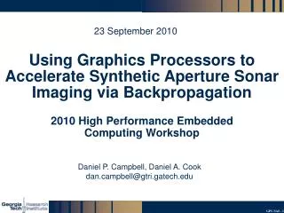
23 September 2010. Using Graphics Processors to Accelerate Synthetic Aperture Sonar Imaging via Backpropagation. 2010 High Performance Embedded Computing Workshop. Daniel P. Campbell, Daniel A. Cook dan.campbell@gtri.gatech.edu. Sonar Imaging via Backpropagation.

E N D
23 September 2010 Using Graphics Processors to Accelerate Synthetic Aperture Sonar Imaging via Backpropagation 2010 High Performance Embedded Computing Workshop Daniel P. Campbell, Daniel A. Cook dan.campbell@gtri.gatech.edu
Sonar Imaging via Backpropagation As the sonar passes by the scene, it transmits pulses and records returns. Each output pixel is computed by returns from the pulses for which it is within the beamwidth (shown in red). A typical integration path is shown in yellow. Forward Travel
Backpropagation Backpropagation is the simplest synthetic aperture image reconstruction algorithm for each output pixel: Find all pulses containing reflections from that location on the ground Find recorded samples at each round-trip range Inner product with expected reflection Sum all of these data points end
Backpropagation – Practical Advantages Procedure Attempt to fly a perfectly straight line Compensate for unwanted motion Form image using Fourier-based method backpropagation Register and interpolate image onto map coordinates Algorithmic simplicity Easier to code and troubleshoot Less accumulated numerical error Flexibility Can image directly onto map coordinates without the need for postprocessing (including bathymetric maps) Expanded operating envelope Can form imagery in adverse environmental conditions and during maneuvers
Sonar vs. Radar Typical SAS range/resolution: 100m/3cm Typical SAR range/resolution: 10km/0.3m SAS and SAR are mathematically equivalent, allowing the same code to be used for both The sensor is in continual motion, so it moves while the signal travels to and from the ground Light travels 200,000 times faster than sound, so SAR processing can be accelerated by assuming the platform is effectively stationary for each pulse.
Sonar vs. Radar In general, the sensor is at a different position by the time the signal is received (above). If the propagation is very fast (i.e., speed of light), then the platform can be considered motionless between transmit and receive (below).
Advantages of Backpropagation FFT-based reconstruction techniques exist Require either linear or circular collections Only modest deviations can be compensated Requires extra steps to get georeferenced imagery Backpropagation is far more expensive, but is the most accurate approach No constraints on collection geometry: can image during maneuvers Directly produces imagery located on any map coordinates desired
Minimum FLOPs Range out 9 Estimated r/t time 1 Beam Check 5 Final receiver position 65 Final platform orientation 6 Construct platform final R 35 Apply R 15 Add platform motion 9 Range In 9 Range->Bin 2 Sample & Interpolate 9 Correlate with ideal reflector 9 Accumulate 2 Total 111 Not needed for Radar
GPU Backpropagation • GTRI SAR/S Toolbox, MATLAB Based • Multiple image formations • Backpropagation too slow • GPU Accelerated plug-in to MATLAB toolbox • CUDA/C++ • One output pixel per thread • Stream groups of pulses to GPU memory • Kernel invocation per pulse group
Direct Optimization Considerations • Textures for clamped, interpolated sampling • 2-D blocks for range (thus cache) coherency • Careful control of register spills • Shared memory for (some) local variables • Reduced precision transcendentals • Recalculate versus lookup • Limit index arithmetic
GPU Ocelot Courtesy, Computer Architecture and Systems Laboratory, Georgia Tech http://www.ece.gatech.edu/research/labs/casl/index.html G. Diamos, A. Kerr, S. Yalamanchili, and N. Clark, “Ocelot: A Dynamic Optimizing Compiler for Bulk Synchronous Applications in Heterogeneous Systems,” IEEE/ACM International Conference on Parallel Architectures and Compilation Techniques, September 2010.
Productivity Tools for Hybrid Systems • Debugging • Memory race detection • Bounds checks • Profiling/Performance Tuning • Alignment behavior • Control flow behavior • Inter-thread data flow • Integration with Front-End profiling tools • GLIMPSES (S. Pande) • Ocelot Dynamic Execution Infrastructure
Ocelot Findings 82.25 FLOPS per pixel*pulse, too high a = calc1(); b = calc2(); if (a<constant) {… 25% Speedup Did not expect any! • tyx = ThreadIdx.x * BLOCK • + ThreadIdx.y; • share[tyx] = foo; • 5% Speedup
Performance – Alternate Configurations • 3936 x 3936 Image from 3936 pulses • Alternate configurations not optimized • GTX 480
Future Work • Further optimization • Reoptimize for Fermi • Tune for multi-GPU • Multi-node • Improve error handling, edge cases, etc. • Backpropagation server