Download
1 / 17
180 likes | 301 Views
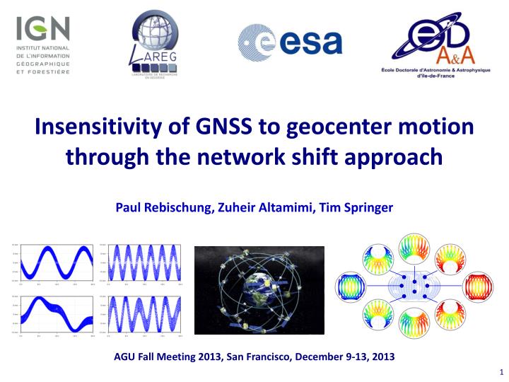
Insensitivity of GNSS to geocenter motion through the network shift approach Paul Rebischung, Zuheir Altamimi, Tim Springer AGU Fall Meeting 2013, San Francisco, December 9-13, 2013. Observing geocenter motion with GNSS. Degree-1 deformation approach (Blewitt et al., 2001):

E N D
Insensitivity of GNSS to geocenter motion through the network shift approachPaul Rebischung, Zuheir Altamimi, Tim SpringerAGU Fall Meeting 2013, San Francisco, December 9-13, 2013
Observing geocenter motion with GNSS • Degree-1 deformation approach (Blewitt et al., 2001): • Based on the fact that loading-induced geocenter motion is accompanied by deformations of the Earth’s crust. • Gives satisfying results. • But can only sense non-secular, loading-induced geocenter motion. • Network shift approach: • Weekly AC solutions theoretically CM-centered. • AC → ITRF translations should reflect geocenter motion. • But unlike SLR, GNSS have so far not proven able to reliably observe geocenter motion through the network shift approach. • Why?
Example of network shift results • The translations of the different IGS ACs show various features. • But none properly senses the X & Z components of geocenter motion. — SLR (smoothed) — GPS (ESA) — GPS (ESA, smoothed) Why? Annual signal missed Spuriouspeaksatharmonics of 1.04 cpy
(Multi-) Collinearity • Consider the linear regression model: y = Ax + v = Σ Aixi + v • Ai = ∂y / ∂xi = « signature » of xi on the observations • Collinearity = existence of quasi-dependenciesamong the Ai’s • Consequences: • Some (linear combinations of) parameters cannot be reliably inferred, • are extremely sensitive to any modeling or observation error, • have large formal errors. observations parameters residuals
Variance inflation factor (VIF) • Is the estimation of a particularparameter xi subject tocollinearity issues? • θi = angle between Ai and the hyper-plane Ki containing all other Aj’s • VIFi= 1 / sin²θi • θi= π/2 (VIFi = 1) : xi is uncorrelated with any other parameter. • θi → 0 (VIFi → ∞): xi tends to be indistinguishable from the other parameters. • If yes, why? • The orthogonal projection αi of Ai on Ki corresponds to the linear combination of the xj’s which is the most correlated with xi.
Mathematicaldifficulties • Geocenter coordinates are not explicitly estimated parameters. • They are implicitly realized through station coordinates. • Extend previous notions to such « implicit parameters ». • There are perfect orientation singularities. • Extend previous notions so as to handle singularities supplementedby minimal constraints. • The whole normal matrix is not available. • Clock parameters are either reduced or annihilated by formingdouble-differenced observations. • Practical collinearity diagnosis (next slide)
Practicaldiagnosis • Simulate « perfect » observations x0→ y0 • Introduce a 1 cm error on the Z geocenter coordinate:x1=x0+[0, 0, 0.01, …, 0, 0, 0.01, 0, …0]T • Re-compute observations → y1 • Solve the constrained LSQ problem: (How can the introduced geocenter error be compensated / absorbed by the other parameters?) → x2, y2 0) 1) 2)
« Signature » of a geocenter shift · impact on a particular observation — epochmean impact • From the satellite point of view: GPS LAGEOS δZgc = 1 cm δXgc = 1 cm
1st issue: satellite clock offsets • Satellite clocks ↔ constant per epoch and satellite → The epoch mean geocenter signature is 100% absorbable by (indistinguishable from) the satellite clock offsets. → The GNSS geocenter determination can only rely on a 2nd order signature. • In case of SLR : • The epoch mean signatures of Xgc and Ygc are directly observable. → No collinearity issue for Xgc and Ygc (VIF ≈ 1) • The epoch mean signature of Zgc is absorbable by the satellite osculating elements. → Slight collinearity issue for Zgc (VIF ≈ 9)
2ndordergeocenter signature δZgc = 1 cm δXgc = 1 cm • 2nd issue: collinearity with station parameters • Positions, clock offsets, tropospheric parameters
So what’sleft? • δXgc = 1 cm: From the point of view of a satellite… …and of a station • VIF > 2000 for the 3 geocenter coordinates!(More than 99.96% of the introduced signal could be absorbed.) · impact on an observation, before compensation · impact on an observation, after compensation
Role of the empiricalaccelerations • The insensitivity of GNSS to geocenter motion is mostly due to the simultaneous estimation of clock offsets and tropospheric parameters. • The ECOM empirical accelerations only slightly increase the collinearity of theZ geocenter coordinate. • This increase is due to the simultaneous estimation of D0, BC and BS:
Conclusions (1/2) • Current GNSS are barely sensitive to geocenter motion. • The 3 geocenter coordinates are extremely collinear with other GNSS parameters, especially satellite clock offsets and all station parameters. • Their VIFs are huge (at the same level as for the terrestrial scale when the satellite z-PCOs are estimated). • The GNSS geocenter determination can only rely on a tiny 3rd order signal. • Other parameters not considered here (unfixed ambiguities) probably worsen things even more (cf. GLONASS).
Conclusions (2/2) • The empirical satellite accelerations do not have a predominant role. • Contradicts Meindl et al. (2013)’s conclusions • What can be done? • Reduce collinearity issues(highly stable satellite clocks?) • Reduce modeling errors(radiation pressure, higher-order ionosphere…) • Continue to rely on SLR…
Thanks for your attention!For more:Rebischung P, Altamimi Z, Springer T (2013) A collinearity diagnosis of the GNSS geocenter determination. Journal of Geodesy. DOI: 10.1007/s00190-013-0669-5
Parameter response to δZgc = 1 cm Network distortion: ZWDs:(as a function of time, for each station) And theirmeans:(as a function of latitude) → Explains the significantcorrelationsbetweenorigin & degree-1 deformationsobserved in the IGS AC solutions Station clock offsets:(as a function of time, for each station) And theirmeans:(as a function of latitude) Tropo gradients:(as a function of latitude) N/S gradients W/E gradients
Zgc collinearity issue in SLR • δZgc = 1 cm: • This slight collinearity issue probably contributes to the lower qualityof the Z component of SLR-derived geocenter motion. • To be further investigated… • The epochmean signature of δZgciscompensated by a periodic change of the orbit radius obtainedthrough: • VIF ≈ 9.0 · impact on an observation, before compensation · impact on an observation, after compensation — radial orbitdifference