Download
1 / 17
170 likes | 347 Views
Spectroscopy. Spectral lines The Fraunhofer spectrum Charlotte Moore Sitterly (Allen!) Multiplet table Rowland table Formalism of spectroscopy. Quantum Numbers of Atomic States. Principal quantum number n defines the energy level Azimuthal quantum number l

E N D
Spectroscopy • Spectral lines • The Fraunhofer spectrum • Charlotte Moore Sitterly (Allen!) • Multiplet table • Rowland table • Formalism of spectroscopy
Quantum Numbers of Atomic States • Principal quantum number n defines the energy level • Azimuthal quantum number l • states with l=0 called s states • states with l=1 called p states • states with l=2 called d states • states with l=3 called f states • “orbits” of s states become more eccentric as n increases • Electron transitions take place between adjacent angular momentum states (i.e. Dl=1) • “sharp series” lines from p to higher s states • “principal series” lines from s to higher p states • “diffuse series” lines from p to higher d states • “fundamental series” lines from d to higher f states • The first line(s) of the principal series (s to p) are called resonance lines since it involves the ground level • In alkali metals, the p, d, and f energy levels are doubled (e.g. the Na D lines) due to the coupling between the magnetic moment of the orbital motion and the spin of the electron (the quantum number s, which can be +1/2 or –1/2
Spectroscopic Notation • The total angular momentum quantum number is j = l +S* • For s states, j=1/2 • For p states, j=1/2 or j=3/2 • Electron levels are designated by the notation “n2(L)J” • n is the total quantum number • The superscript 2 indicates the levels are doubled • L is the azimuthal quantum number (S,P,D,F) • J denotes the angular momentum quantum number • For the sodium ground level is 3s2S1/2 • The two lowest p levels are 3p2P1/2 and 3p2P 3/2 • The Na D lines are described • 3s2S½ - 3p2P3/2 l5889.953 and 3s2S½ - 3p2P1/2l5895.923 * This is a different S than the s state!
More Spectroscopic Vocabulary • The Pauli exclusion principle requires that two s-electrons in the same state must have opposite spin • Therefore S=0 and these are called “singlet” states • The ground state of He is a singlet state – 1S0 • The superscript 1 means singlet • The subscript 0 means J=0 • In the first excited state of He, one electron is in the 1s state, and the second can be in either the 2s or the 2p state. • Depending on how the electrons’ spins are aligned, these states can either be singlets or triplets • Electrons can only jump between singlet states or between triplet states
It goes on and on and on…. • The state of the electrons is described with a term for each electron above the closed shell. • For carbon atoms, “1s22s22p2”says there are • 2 electrons in the 1s state • 2 electrons in the 2s state • 2 electrons in the 2p state
Allowed and Forbidden Transitions • Transitions with Dl=1 and DJ=1 and 0 are allowed (except between J=0 and J=0) • Other transitions are forbidden • For some electron states there are no allowed transitions to lower energy states. Such levels are called metastable • The situation is more complex in atoms with more electrons • A multiplet is the whole group of transitions between two states, say 3P-3D
Grotrian Diagram for He • Struve and Wurm 1938, ApJ
Spectral Line Formation • Classical picture of radiation • Intrinsic vs. extrinsic broadening mechanisms • Line absorption coefficient • Radiative transfer in spectral lines
Spectral Line Formation-Line Absorption Coefficient • Radiation damping (atomic absorptions and emissions aren’t perfectly monochromatic – uncertainty principle) • Thermal broadening from random kinetic motion • Collisional broadening – perturbations from neighboring atoms/ions/electrons) • Hyperfine structure • Zeeman effect
Classical Picture of Radiation • Photons are sinusoidal variations of electro-magnetic fields • When a photon passes by an electron in an atom, the changing fields cause the electron to oscillate • Treat the electron as a classical harmonic oscillator: mass x acceleration = external force – restoring force – dissipative • E&M is useful!
Atomic Absorption Coefficient • N0 is the number of bound electrons per unit volume • the quantity n-n0 is the frequency separation from the nominal line center • the quantity e is the dielectric constant (e=1 in free space) • and g=g/m is the classical damping constant The atomic absorption coefficient includes atomic data (f, e, g) and the state of the gas (N0), and is a function of frequency. The equation expresses the natural broadening of a spectral line.
The Classical Damping Constant • For a classical harmonic oscillator, • The shape of the spectral line depends on the size of the classical damping constant • For n-n0 >> g/4p, the line falls off as (n-n0)-2 • Accelerating electric charges radiate. • and • is the classical damping constant (l is in cm) The mean lifetime is also defined as T=1/g, where T=4.5l2
Line Absorption with QM • Replace g with G! • Broadening depends on lifetime of level • Levels with long lifetimes are sharp • Levels with short lifetimes are fuzzy • QM damping constants for resonance lines may be close to the classical damping constant • QM damping constants for other Fraunhofer lines may be 5,10, or even 50 times bigger than the classical damping constant
The Classical Line Profile • Look at a thin atmospheric layer between t2 (the deeper layer) and t1 • The line profile is proportional to kn • At line center n=n0, and • Half the maximum depth occurs at (n-n0)=g/4p • In terms of wavelength • Very small – and the same for ALL lines!
An example… • The Na D lines have a wavelength of 5.9x10⁻⁵ cm. g = 6.4 x 10⁷ sec-1 • The absorption coefficient per gram of Na atoms at a distance of 2A from line center can be calculated: • n0-n = 1.7 x 10¹¹ sec-1 and N = 1/m = 2.6 x 10²² atoms gm-1 • Then k = 3.7 x 10⁴f • and f=2/3, so k = 2.5 x 10⁴ per gram of neutral sodium
The Abundance of Sodium • In the Sun, the Na D lines are about 1% deep at a distance of 2A from line center • Use a simple one-layer model of depth x (the Schuster-Schwarzschild model) • Or krx=0.01, and rx=4x10⁻⁷ gm cm-2