Download
1 / 67
680 likes | 1.04k Views
Co-Optimizations for Electricity and Natural Gas Sectors. Introduction to Concepts, Theory, Working Examples. Dr. Randell M. Johnson, P.E. October 28 th & 29 th , 2013. Co-Optimizations for Natural Gas and Electric Sectors. Optimizations Methods

E N D
Co-Optimizations for Electricity and Natural Gas Sectors Introduction to Concepts, Theory, Working Examples Dr. Randell M. Johnson, P.E. October 28th & 29th, 2013
Co-Optimizations for Natural Gas and Electric Sectors • Optimizations Methods • Co-Optimization Generation and Transmission Expansion • Co-Optimization of Energy and Ancillary Services • Co-Optimization Electric and Nat Gas Production Cost • Co-Optimization of Nat Gas and Electric Markets with Co-Optimization of Ancillary Services • Co-Optimization Electric and Nat Gas Capacity Expansion • Integrated Datasets
PLEXOS Optimization Methods • Linear Relaxation - The integer restriction on unit commitment is relaxed so unit commitment can occur in non-integer increments. Unit start up variables are still included in the formulation but can take non-integer values in the optimal solution. This option is the fastest to solve but can distort the pricing outcome as well as the dispatch because semi-fixed costs (start cost and unit no-load cost) can be marginal and involved in price setting • Rounded Relaxation - The RR algorithm integerizes the unit commitment decisions in a multi-pass optimization. The result is an integer solution. The RR can be faster than a full integer optimal solution because it uses a finite number of passes of linear programming rather than integer programming. • Integer Optimal - The unit commitment problem is solved as a mixed-integer program (MIP). The unit on/off decisions are optimized within criteria. • Stochastic Programing - The goal of SO is to find some policy that is feasible for all (or almost all) of the possible data instances and maximize the expectation of some function of the decisions and the random variables Energy Exemplar
Stochastic Optimization (SO) • Fix perfect foresight issue • Monte Carlo simulation can tell us what the optimal decision is for each of a number of possible outcomes assuming perfect foresight for each scenario independently; • It cannot answer the question: what decision should I make now given the uncertainty in the inputs? • Stochastic Programming • The goal of SO is to find some policy that is feasible for all (or almost all) of the possible data instances and maximize the expectation of some function of the decisions and the random variables • Scenario-wise decomposition • The set of all outcomes is represented as “scenarios”, the set of scenarios can be reduced by grouping like scenarios together. The reduced sample size can be run more efficiently
Stochastic Variables • Set of uncertain inputs ω can contain any property that can be made variable in PLEXOS: • Load • Fuel prices • Electric prices • Ancillary services prices • Hydro inflows • Wind energy, etc • Number of samples S limited only by computing memory • First-stage variables depend on the simulation phase • Remainder of the formulation is repeated S times
20 Sample input distribution for variables Wind Solar No Solar Low Wind High load Peak Load Load
SO Theory, Continued • Where the first (or second) stage decisions must take integer values we have a stochastic integer programming (SIP) problem • SIP problems are difficult to solve in general • Assuming integer first-stage decisions (e.g. “how many generators of type x to build” or “when do a turn on/off this power plant”) we want to find a solution that minimises the total cost of the first and second stage decisions • A number of solution approaches have been suggested in the literature • PLEXOS uses scenario-wise decomposition ...
SO Theory, Continued 2-stage SIP Formulation
SO Theory, Continued Scenario wise Decomposition of 2-stage SIP Formulation
H3 H1 H2 H3 H2 M3 H1 H2 M3 H1 H3 H1 M2 H3 M2 M3 H1 M2 M3 Initial “high” L3 H1 M2 L3 P(1) M1 H2 H3 H3 M1 H2 H3 H2 M1 H2 M3 P(2) M3 M1 H2 M3 P(3) M1 M2 H3 H3 M1 M2 H3 M1 M2 M3 M1 M2 M3 M1 M2 M3 M1 M2 L3 L3 M1 M2 L3 L1 M2 H3 M3 M1 L2 M3 L2 L1 M2 M3 Initial “mid” L3 M1 L2 L3 Initial Problem Scenarios Sample Reduction L1 M2 L3 H3 L1 M2 H3 p(9) L1 M2 M3 M2 M3 L1 M2 M3 L2 L3 L1 M2 L3 M3 L1 M2 M3 L2 Initial “low” L3 L1 L2 L3
Day-ahead Unit Commitment, Continued Stochastic Optimisation: Two stage scenario-wise decomposition Stage 1: Commit 1 or 2 or none of the “slow” generators Stage 2: There are hundreds of possible wind speeds. For each wind profile, decide the optimal commitment of the other units and dispatch of all units RESULT: Optimal unit commitment for “slow” generator
Overview: Generation Transmission Expansion Planning • Focus on long-term studies with decision variables spanning many years: • Co-optimize generation new builds and retirements with: • Transmission line builds e.g. AC or DC lines; and • Transmission interface upgrades; • Physical contract purchases (generation or load)
Objective Function • Object function minimizes (expected value of) the net present value (NPV): • Cost of new builds: • Generator, DC Line, AC Line, Interface, Physical Contract • Cost of retirements: • Generator, DC Line • Fixed operating costs • Variable operating (production) costs • Net cost of external market trades
Optimal Decisions under Uncertainty • New investments: • Where? • Location • When? • Timing • How much? • Sizing • Retirements… • When? • Timing • How much? • Number of units • Uncertainties: • Load • Fuel prices • Hydro inflows • Wind energy • Outages • etc • Constraints: • Reliability (LOLP) • Emissions • Fuels • etc
Objective Function Components • For any combination of expansion decisions x we have two types of costs: • Capital costs C(x): • Cost of new builds • Cost/savings from retirements • Production costs P(x): • Cost of operating the system with any given set of existing and new builds and transmission network • Notional cost of unserved energy
Optimization Objective: Minimize net present value of forward-looking costs (i.e. capital and production costs) Cost $ Total Cost = C(x) + P(x) Investment cost/ Capital cost C(x) Production Cost P(x) Minimum cost plan x Investment x
Illustrative Formulation Generation Transmission Expansion Co-Optimization This simplified illustration shows the essential elements of the mixed integer programming formulation. Build decisions cover generation, and transmission as does supply and demand balance and shortage terms. The entire problem is solved simultaneously, yielding a true co-optimized solution.
Algorithms • Chronological or load duration curves • Large-scale mixed integer programming solution • Deterministic, Monte Carlo; or • Stochastic Optimization (optimal decisions under uncertainty)
Generation Expansion Capabilities • Building new generating plant • Retiring existing generating plant • Multi-stage projects e.g. GT before CCGT • Thermal or hydro with storage • Multi-annual emission caps • Fuel-supply policies and constraints • Pumped storage • Other renewables: • Wind, solar, wave, etc
Transmission Expansion Capabilities • Building new DC transmission lines • Retiring existing DC transmission lines • Building new AC transmission lines: • Dynamic changes in impedance matrix • Multi-stage transmission projects • Transmission Interface expansion
Ancillary Services Products • Integration of the intermittency of renewables requires study of Co-Optimization of Ancillary Services and true co-optimization of Ancillary services is done on a sub-hourly basis in real time markets • More and more the last decade, it has been recognised that AS and Energy markets are closely coupled as the same resource and same capacity have to be used to provide multiple products when justified by economics. • The capacity coupling for the provision of Energy and AS, calls for joint optimisation of Energy and AS markets that differs from market to market due to different regional reliability standards and operational practises.
Ancillary Service Products in Wholesale Markets Reliable and Secure System Operation requires the following product and Services (not exhausted): Energy Regulation & Load Following Services – AGC/Real time maintenance of system’s phase angle and balancing of supply/demand variations. Synchronised Reserve – 10 min Spinning up and down Non-Synchronised Reserve – 10 min up and down Operating Reserve – 30 min response time Voltage Support – Location Specific Black Start – (Service Contracts) Co-Optimization
Solving SC UC/ED using MIP • Unit Commitment and Economical Dispatch can be formulated as a linear problem (after linearization) with integer variables of generator on-line status Minimize Cost = generator fuel + VOM cost + generator start cost + contract purchase cost – contract sale saving + transmission wheeling + energy / AS / fuel / capacity market purchase cost – energy / AS / fuel / capacity market sale revenue Subject to: • Energy balance constraints • Operation reserve constraints • Generator and contract chronological constraints: ramp, min up/down, min capacity, etc. • Generator and contract energy limits: hourly / daily / weekly / … • Transmission limits • Fuel limits: pipeline, daily / weekly/ … • Emission limits: daily / weekly / … • Others
Security Constrained Unit Commit /Economic Dispatch • SCUC / ED consists of two applications: UC/ED and Network Applications (NA) • SCUC / ED is used in many power markets in the world include CAISO, MISO, PJM, etc. Energy-AS Co-optimization using Mixed Integer Programming (MIP) enforces resource chronological constraints, transmission constraints passed from NA, and others. Solutions include resource on-line status, loading levels, AS provisions, etc. Resource Schedules in 24 hours for DA simulations, or in sub-hourly for RT simulations DC-Optimal Power Flow (DC-OPF) solves network power flow for given resource schedules passed from UC/ED enforces transmission line limits enforces interface limits enforces nomograms Network Applications (NA) Unit Commitment / Economic Dispatch (UC/ED) Violated Transmission Constraints
Flow Diagram of Sequential DA/RT Modelling and Simulation Sequential DA/RT is Optional Additional Feature for Simulation
PLEXOS Example: Sub-Hourly Energy and Ancillary Services Co-Optimization
PLEXOS Base Model Generation Result • Peaking plant in orange operating at morning peak • Some displacement of hydro to allow for ramping • Variable wind in green
Spinning Reserve Requirement • CCGT now runs all day to cover reserves and energy • Coal plant 2 also online longer • Oil unit not required • Less displacement of hydro generation for ramping
PLEXOS higher resolution dispatch – 5 Minute Sub-Hourly Simulation • Oil unit required at peak for increased variability • Increased displacement of base load to cover for ramping constraints
Energy/AS Stochastic Co-optimisation!!! So far the model example has had perfect information on future wind and load requirements. Uncertainty in our model inputs should affect our decisions – Stochastic optimisation (SO) • The goal of SO then is to find some policy that is feasible for all (or almost all) the possible data instances and maximise the expectation of some function of the decisions and the random variables What decision should I make now given the uncertainty in the inputs?
Energy/AS Stochastic Co-optimisation • Even though load lower (wind unchanged) more units must be committed to cover the possibility of high load and low wind • These units must then operate at or above Minimum Stable Level
Illustrative Formulation of Co-Optimization of Natural gas and Electricity Markets • Objective: • Co-Optimization of Natural Gas Electricity Markets • Minimize: • Electric Production Cost + Gas Production Cost + Electric Demand Shortage Cost + Natural Gas Demand Shortage Cost • Subject to: • [Electric Production] + [Electric Shortage] = [Electric Demand] + [Electric Losses] • [Transmission Constraints] • [Electric Production] and [Ancillary Services Provision] feasible • [Gas Production] + [Gas Demand Shortage] = [Gas Demand] + [Gas Generator Demand] • [Gas Production] feasible • [Pipeline Constraints] • others
PLEXOS Example: Co-Optimization of Natural Gas and Electricity Markets for simplified northeast model
New England and New York Markets • Created a simple dataset to proxy the NY and New England electricity and natural gas markets. • Several simplifying assumptions: • Assumed aggregation of gas production • Simplified both the natural gas and electricity network in New York State and New England. • Simplified the complexity of generators and interconnections. Integrated Gas and Electric Model
Northeast Market Simplified Assumptions • Zonal electric market with limited transmission • New York 3 zones: New York City and Long Island; Upstate NY and Western NY. • New England 3 zones: North (ME, NH, VT); and West (MA, CT & RI); Central (eastern MA). • 4 natural gas production regions: • Alberta Canada with an interconnection at the Niagara Hub; Waddington and Montreal; • Gulf coast with an interconnection in New Jersey; • Shale Production in Mid-Western States with interconnection in Pennsylvania; and • A small natural gas production in upstate New York. • 2 Natural Gas Markets: New York and New England. • 5 adjoining electrical markets: • PJM; NY, Ontario; Quebec and New England. • Daily natural gas load based on EIA monthly demand. Integrated Gas and Electric Model
Simplified Combined Electric & Natural Gas Model Gas Montreal Electric Montreal Wadding ton North NE To Alberta Niagara Hub North NE Upstate West Ontario West NE West Upstate Central NE Central NE West NE PJM West Leidy NJ Hub NYC PJM East NYC To Shale To Gulf
Simplified Model Inputs/Results NY and New England Gas Demand Natural gas demand (non-generation) provided by EIA. Generation gas demand calculated by PLEXOS. Integrated Gas and Electric Model
Simplified Model Inputs/Results Northeast Natural Gas Prices Natural Gas prices at Leidy, Niagara Hub and Transco Z6 are used as the production costs for the natural gas into NY and New England. Citygate prices are calculated by PLEXOS. Integrated Gas and Electric Model
Simplified Model Results Daily Pipeline Flows Natural Gas production serving the Northeast: NY, Shale; Gulf; and Canada production. Calculated by PLEXOS. Integrated Gas and Electric Model
Simplified Model Results NY Electrical Load Integrated Gas and Electric Model
Simplified Model Results New England Electrical Load Integrated Gas and Electric Model
Simplified Model Results NY Electric LBMP Nat Gas Network Constraints • Electric Prices for • NYC (Zones J-K); • Upstate (Zones F-I); • West (Zones A-E). • Prices in Winter influenced by natural gas shortages. Summer prices reflect electric constraints calculated by PLEXOS. Electrical Network Constraints Integrated Gas and Electric Model
Simplified Model Results ISONE LMP Electric Prices for ISONE. Prices in Winter influenced by natural gas shortages. Summer prices reflect shortages calculated by PLEXOS. Nat Gas Network Constraints Electrical Network Constraints