Download
1 / 68
680 likes | 1.08k Views
Introduction to Scientific Visualization in the WestGrid Environment Jon Johansson What is Scientific Visualization? convert scientific data into visual form use computer to process data numerical algorithms such as marching cubes to extract features

E N D
Introduction to Scientific Visualization in the WestGrid Environment Jon Johansson
What is Scientific Visualization? • convert scientific data into visual form • use computer to process data • numerical algorithms such as marching cubes to extract features • add color, lights, camera view (create a 3D scene) • graphics techniques to render • the data sets can be large – many gigabytes or more • resulting image is presented to the human visual processing system for the direct analysis and interpretation of the information
What is Scientific Visualization? • generally deals with data that has a natural geometric structure • MRI, CAT data (measured) • weather simulations (computed)
What is Scientific Visualization? • the key point is that we can understand data in a picture much better than we can understand a bunch of numbers • WestGrid resources can generate a lot of numbers!!
What is Scientific Visualization? • use well understood algorithms to extract features from data sets • goals • understand the data (exploration) • interactively examine the data looking for the parts that are interesting • communicate the data to peers • publications • conferences
What is Scientific Visualization? • once we find interesting structures in the data we have the freedom to arrange • colors • lights • transparency • camera views • this should clarify what we are looking at
WestGrid Visualization Resources • WestGrid provides a visualization server located at Simon Fraser University • the machine can be accessed as: • hydra.westgrid.ca • vizserver.westgrid.ca • IP address: 206.12.24.8 • Hydra is an SGI Onyx UltimateVision graphics supercomputer • 24 processors • 14 GB RAM • 10 graphics pipes
WestGrid Visualization Resources • You should have access to hydra automatically by being granted access to WestGrid resources • Info about accounts: • http://www.westgrid.ca/support//About_Accounts • Apply for an account at: • http://www.westgrid.ca/support//Applying_for_an_Account
WestGrid Visualization Resources Web links for more information: • WestGrid Collaboration/Visualization • http://www.westgrid.ca/collabvis/visualization/ • Visualization Server Usage page • http://www.westgrid.ca/collabvis/visualization/vizserver_software.php • SFU Visualization Server Site • http://www.westgrid.ca/support_old/site/site-viz.php
OpenGL Vizserver • SGI Vizserver is client-server software that allows you to run fully hardware-accelerated graphics applications on a remote machine and have images delivered to your desktop • the server is installed on • hydra.westgrid.ca • the client is installed on your workstation
OpenGL Vizserver • OpenGL VizServer • the server software runs on the WestGrid Visualization Server machine • the client runs on the users desktop machine • http://www.sgi.com/products/software/vizserver/ • there are currently 5 licenses for the Vizserver software on hydra
OpenGL Vizserver • Application-transparent • OpenGL Vizserver runs existing OpenGL® API-based applications without modification • Shared application control • OpenGL Vizserver instantly turns existing stand-alone applications into collaborative applications with up to five remote sites sharing control of a single interactive application
OpenGL Vizserver • Platform/system independent • OpenGL Vizserver gives existing workstations, personal computers, and even wireless handheld devices the power of a Silicon Graphics Prism or SGI Onyx family system, as well as direct interaction with experts on Silicon Graphics workstations.
OpenGL Vizserver • you can run nearly any graphics or visualization application on the remote SGI host (hydra.westgrid.ca), and have the resulting imagery delivered to your desktop • the client machine simply decompresses and displays the image created by the server
OpenGL Vizserver • why the Vizserver approach is better: • X doesn't support hardware accelerated 3D graphics • OpenGL function calls are passed to the graphics card on your desktop • the X protocol is horribly inefficient • Vizserver uses a much more streamlined (custom) protocol to move events and payload image data • data compression is available • Vizserver lets multiple users interact simultaneously with a single application running on the graphics server • each connection has a dedicated graphics pipe
OpenGL Vizserver • OpenGL Vizserver clients are available for • SGI® IRIX® OS-based systems, such as Silicon Graphics Octane2, Silicon Graphics Fuel, Silicon Graphics® O2+™, and the SGI Onyx family • Linux® • Solaris™ • Windows NT®, Windows® 2000, Windows® XP, and Windows® XP Tablet PC Edition • Mac OS X
OpenGL Vizserver • the OpenGL Vizserver client is a free download from the SGI website • https://support.sgi.com/login • note that you must create a Supportfolio ID to be able to download the client • this is free
Connection to Hydra • you need to create an SSH tunnel to hydra to be able to use it. • from a Linux/Unix machine: • ssh -L 7051:hydra.westgrid.ca:7051 -N username@hydra.westgrid.ca • replace “username” with your WestGrid username and you will be prompted for your password • 7051 is the port that vizserver uses to make connections
Connection to Hydra • you will need to set an environment variable to be able start a vizserver session: • VSX_SESSION_HOST = hydra.westgrid.ca • launch the vizserver client • connect to “localhost” not to hydra • the connection is handled by the tunnel • you still need to authenticate to Hydra with your WestGrid username and password. • http://www.westgrid.ca/collabvis/documents/vizserver_tunnel.pdf
Connection to Hydra Sample session start • set up the SSH tunnel • ssh -L 7051:hydra.westgrid.ca:7051 -Nusername@hydra.westgrid.ca • set the environment variable (Bash shell) • export VSX_SESSION_HOST=hydra.westgrid.ca • launch the client • vizserver -h localhost
OpenGL Vizserver • Sample session start (cont.) • enter your WestGrid user id and password to login to hydra • start a session • select parameters for the session • launch applications from the vizserver console window
SSH tunneling • also called “port forwarding” or “port mapping” • forward a network port from one network node to another • used to carry insecure network traffic over the Internet in a secure way • users outside a firewall can access a service inside the firewall
SSH tunneling • ssh connects using port 22 • connection is encrypted and secure • vizserver connects using port 7051 • connection is not encrypted • to make a vizserver session secure, wrap the vizserver session inside ssh
SSH tunneling • on the source machine • ssh listens for packets addressed to port 7051 • all those packets are encrypted and addressed to the destination using port 22 • on the destination machine • when the packets are received, ssh decrypts them • packets are then sent to the destination port
SSH tunneling • We can use a GUI and manually assign port forwarding • port 7051 on localhost is forwarded to 7051 on the remote host • this is an “outgoing” tunnel • we don’t need an incoming (reverse) tunnel for port 7051 - only an outgoing tunnel to the server • our big concern is that the username and password used to authenticate to hydra be encrypted
Scientific Visualization • Having opened a connection to hydra we would like to use a visualization application – what’s available?
Viz Packages • OpenDX, VTK are AVS use a pipelined, component-based architecture • a user can quickly assemble modular software components into a “finished application.” • these systems are flexible in the sense that components can be combined in a multitude of ways, thereby allowing an application developer to accomplish a wide variety of visualization tasks • they are extensible as they offer the means for developers to add new components to the system, thereby extending the system’s functionality
Scientific Visualization • to be able to run OpenDX on hydra: • set the environment variable DXROOT to • setenv DXROOT /usr/local/dx (tcsh) • export DXROOT=/usr/local/dx (bash) • add the following directory to your library path • setenv LD_LIBRARY_PATH {LD_LIBRARY_PATH}:/usr/local/lib/ (tcsh)
Scientific Visualization • In order to create a visualization: • import your data into the package • explore the data looking for the interesting features • lots of work here • having found interesting features set up the view to show them clearly. Select: • colors/surface properties • camera view • lights (these have some properties to adjust) • export images/animations
Scientific Visualization • color choice can help to clarify a visualization • a handy guide is the online paper “A Rule-based Tool for Assisting Colormap Selection” by Lawrence D. Bergman, Bernice E. Rogowitz and Lloyd A. Treinish, all from IBM • http://www.research.ibm.com/dx/proceedings/pravda/index.htm • lots of interesting references at the end
Scientific Visualization • another very nice online publication is “How NOT to Lie with Visualization” by Bernice E. Rogowitz and Lloyd A. Treinish, from IBM • http://www.research.ibm.com/dx/proceedings/pravda/truevis.htm • PRAVDA is intellectual property (IBM’s) separate from OpenDX and isn’t freely available • the papers are still worth reading
Scientific Visualization Source: http://www.research.ibm.com/dx/proceedings/pravda/truevis.htm
Sample Data Set • We have the electric potential due to a dielectric cylinder introduced into a constant electric field E0 • the parameters I used are: • E0 = 50 V/m • dielectric constant = 5 • Rcyl = 10 m • -50 m ≤ x, y, z ≤ 50 m
OpenDX Data Import • a data file might consist of ascii values, each line containing 4 values … -8.50000000 14.72243186 48.00000000 326.96078431 -8.50000000 14.72243186 49.00000000 326.96078431 -8.50000000 14.72243186 50.00000000 326.96078431 -9.50627936 14.09363873 -50.00000000 365.66830060 -9.50627936 14.09363873 -49.00000000 365.66830060 -9.50627936 14.09363873 -48.00000000 365.66830060 … • it’s important know how the file was written: • row major: for( i = 0; i < nx; i++){ for( j = 0; j < ny; j++){ for( k = 0; k < nz; k++){ fprintf( outfh, "%12.8f %12.8f %12.8f %12.8f \n", x, y, z, V ); } } } • row major is defined by the last index varying the fastest
OpenDX Data Import • We have a data set that has regular spacings in the x, y and z directions • We don’t need to read the coordinates for each point from a file • The general header file to read in this data is: • file = ./pot_cart.dat • grid = 101 x 101 x 101 • format = ascii • interleaving = field • majority = row • header = lines 0 • field = potential • structure = scalar • type = float • dependency = positions • positions = regular, regular, regular, -50.0, 1.0, -50.0, 1.0, -50.0, 1.0 • end
Sample Data Set • the connections between the points are inferred when you tell OpenDX that the data are “row major” • these are Cartesian connections
Sample Data Set • you can also work in non-Cartesian coordinates • the grid is row major in cylindrical coordinates (r, phi, z) • write Cartesian coordinates in the file and connections are inferred from the cylindrical grid
Data Import • Start with a FileSelector module to browse to the general file describing the data set and connect it to an import module which actually does the reading • Double click on the FileSelector to get a widget to browse the file system • When the data is in the package we can start applying algorithms to it and look for interesting features
Components of the visualization • Isovalues of the electric potential • The lower slice shows the electric potential with contour lines to give a sense of the shape change close to the cylinder • Use a slab module to extract a slice of the potential field • Use the Isosurface module to extract contour lines at values • -1750, -1250, -750, -250, 250, 750, 1250, 1750 volts
Components of the visualization • In the Slab module set the parameters: • dimension: “z” • position: 0 • thickness: (0 or 1) • this is the default • The AutoColor module generates a color map so that we have something to see
Components of the visualization • Take the output of the Slab module and attach it to the input of an Isosurface module • The 2D slab data will result in contour lines • Set the isovalues at • -1750, -1250, -750, -250, 250, 750, 1250, 1750 volts • The contour lines are then passed to a Tube module • Set the diameter of the tube to 1.0
Components of the visualization • Electric field lines • The middle slice is color mapped to the magnitude of the electric field and shows some field lines • The lines are diverted in the region of the cylinder • Use the Gradient module and the Compute module to calculate the electric field from the electric potential E = - gradj
Components of the visualization • Use a Slab module to extract a slice of the electric field • Use the Streamline module to extract contour lines at values • The Streamline module needs the vector field as one input, and a set of seed points as the next input • Use the Tube module to produce lines with some thickness
Components of the visualization • Use the Compute module after the gradient to negate the vector components • In the Compute module set “expression” to [-a.x, -a.y, -a.z] • In Slab set • dimension: “z” • position: 50 • thickness: (0 or 1) • this is the default