Download
1 / 40
400 likes | 482 Views
NOVELTY DETECTION THROUGH SEMANTIC CONTEXT MODELLING. Pattern Recognition 45 (2012) 3439–3450. Suet-Peng Yong , Jeremiah D.Deng, MartinK.Purvis. The geographical DB contains a lot of objects as well as scenes and we cannot compare only theirs properties

E N D
NOVELTY DETECTION THROUGH SEMANTIC CONTEXT MODELLING Pattern Recognition 45 (2012) 3439–3450 Suet-Peng Yong , Jeremiah D.Deng, MartinK.Purvis
The geographical DB contains a lot of objects as well as scenes and we cannot compare only theirs properties we need to set up different requirements to detect or discover context relationship between objects.
Detection is an important functionality that has found many applications in information retrieval and processing. The framework starts with image segmentation, followed by feature extraction and classification of the image blocks extracted from image segments. SEMANTIC CONTEXT WITHIN THE SCENE
Contextual knowledge can be obtained from the nearby image data and location of other objects. Semantic context (probability): co-occurrence with other objects and in terms of its occurrence in scenes. Basic information is obtained from training data or from an external knowledge base.
Context information - from a global and local image level. Interactions: pixel, region, object and object-scene interactions. Contextual interactions Local interactions Pixel interactions Region interactions Object interactions Global interactions Object-scene interactions The goal: Integrating context
Pixel based image similarity Let f and g be two gray-value image functions. Histogram basedimage similarity Similar images have similar histograms Warning: Different images can have similar histograms
Local interactions Co-occurrence matrices (spatial context) In image processing, co-occurrence matrices were proposed by Haralick as texture feature representation (local or low-level context). Size 256 X 256, co-occurrence in different directions and different distances. Sparse matrix – evaluation of arrangement inside matrix.
Global interactions The semantic co-occurrence matrices then undergo binarization and principal component analysis for dimension reduction, forming the basis for constructing one-class models on scene categories. *********************************************************************************** An advantage of this approach is that it can be used for novelty detection and scene classification at the same time.
Scenes with similar objects but different context can either be normal or novel: • ‘normal’ scene (b) ‘novel’ scene
From a statistical point of view, novelty detection is equivalent to anomaly detection or outliers detection. Type 1 - to determine outliers without prior knowledge - analogous to unsupervised clustering). Type 2 - is to model both normality and abnormality with pre-trained samples, which is analogous to supervised classification. Type 3 - refers to semi-supervised recognition, where only normality is modelled but the algorithm learns to recognize abnormality.
This approach is focused on semantic analysis of individual scenes and then employ statistical analysis to detect novelty. Anomaly detection in images has been explored in specific domains such as biomedicine and geography. WE ARE INTERESTED NOT IN PIXEL OR REGION LEVEL NOVELTY, BUT IN THE CONTEXT OF THE OVERALL SCENE.
Computational framework The computational framework for image novelty detection and scene classification.
JSEG - Segmentation of color-texture regions in images The essential idea of JSEG is to separate the segmentation process into two independently processed stages, color quantization and spatial segmentation(efficient and effective).
In JSEG, colours in the image are first quantized to some representing classes that are used to separate the regions in the image. Image pixel colours are then replaced by their corresponding colour class labels to form a class-map of the image. Two parameters are involved in the algorithm: a colour quantization threshold and a merger threshold.
By segmenting an image into homogeneous regions, it facilitates detection or classification of theobjects. The segmentation has been done using the JSEG package, with the colour quantization threshold set as 250, and the merger threshold as 0.4.
Eachsegmentimageis further tiledinto b x bpixel blockswhere bЄN. Feature extraction and block labelling. ! Size of block – texture features! smallest segment 31 X 67 b = 25
The main disadvantage of the RGB colour space in applications with natural images is a high correlation betweenits components: about 0.78for rBR (cross correlation between the B and R channel), 0.98 for rRG and 0.94 forrGB Another problem is the perceptual non-uniformity, the low correlation between the perceived difference of two colours and the Euclidian distance in the RGB space.
LUV histograms are found to be robust to resolution and rotation changes. It models human’s perception of colour similarity very well, and is also machine independent. LUV colour space - main goal is to provide a perceptually equal space.
The LUV channels have different ranges: L ( 0 - 100), U (- 134 to 220) and V (- 140 to 122). Same interval - it is 20 bins to the L channel, 70 bins to the U channel, 52 bins to the V channel and standard deviation The LUV histogram feature code thus has 143 dimensions. Haralick texture features (a total of 13 statistical measures can be calculated for each co-occurrence matrix in four directions) μ and Ϭ 26 dimensions 169 dimensions
The Euclidian distance between two colours in the LUV colour space is strongly correlated with the human visual perception. L gives luminance and U and V gives chromaticity values of colour image. Positive value of U indicates prominence of red component in colour image, negative value of V indicates prominence of green component.
Edge Histogram Descriptor Gabor filtering features
Block labelling Classification was done on the segments and also on the image blocks with similar feature extractions the classifier employed is nearest neighbour (1-NN) We can now adopt the LUV and Haralick features and concatenate them together, giving a feature vector of 169 dimensions to represent an image block.
Semantic context modelling To model the semantic context within a scene, we further generate a block label co-occurrence matrix (BLCM) within a distance threshold R. The co-occurrence statistics is gathered across the entire image and normalized by the total number of image blocks. Obviously the variation on the object sizes will affect the matrix values. To reduce this effect, one option is to binarize the values of BLCM elements, with non-zero elements all set to 1.
Image blocks in an ‘elephant’ image and its corresponding co-occurrence matrix. The matrix is read row-column, e.g., a ‘sky’-‘land’ entry of ‘1’indicates there is ‘sky’ block above (or to the left of) ‘land’ block.
The dimension of the BLCM will depend on the number of object classes in the knowledge or database. Sparse matrix, PCA to reduce dimensionality and to concanate rows – 1D feature vector. Building scene classifiers This is not a typical multi-class classification scenario. To build a one-class classifier for each of the scene types, the classifiers need only normally labelled images for training. The method is called ‘Multiple One-class Classification with Distance Thresholding’ (MOC-DT).
Testing of MOC-DT. 1. • Given a query image, calculate its BLCM code and its distance towards • each image group as • 2. If label the image as ‘novel’; otherwise, • assign the scene label c to the image,
Experiments and results The normal image set consists of 335 normal wildlife scenes taken from Google image Search and Microsoft Research (the ‘cow’ image set). Wildlife images usually feature one type of animal in the scene with a few other object classes in background to form the semantic context.
Experiments and results There are six scene types (each followed by the number of instances in each type): ‘cow’ (51), ‘dolphin’ (57), ‘elephant’ (65), ‘giraffe’ (50), ‘penguin’ (55) and ‘zebra’ (57). The distribution of number of images across different scene types is roughly even. The background objects belong to eight object classes: ‘grass’, ‘land’, ‘mount’, ‘rock’, ‘sky’, ‘snow’, ‘trees’ and ‘water’.
Animal and background objects: there are 14 object classes in total.
After segmentation, there are 65000 image blocks obtained in total, and these are used to train the classifiers, 30 ‘normal’ images together with 43 ‘novel’ images to make up a testing image set of 73 images For the classification of image blocks, an average accuracy of 84.6% is achieved in a 10-fold cross validation using a 1-NN classifier.
Block labelling Classification was done on the segments and also on the image blocks with similar feature extractions the classifier employed is nearest neighbour (1-NN) We can now adopt the LUV and Haralick features and concatenate them together, giving a feature vector of 169 dimensions to represent an image block.
90% of all image blocks are set aside to be used to train a classifier each time, which then labels the image blocks of the testing images. Results The semantic context of image scenes are calculated, undergoing binarization and PCA. The BLCM data has a higher dimensionality (196) than the number of images in each scene type (50–65).
The 2-D PCA projection of BLCM data for ‘normal’ images shown with their respective classes.
Global scene descriptor(GSD), Local binary pattern (LBP), Gist [34], BLCM, BLCM with PCA (BLCM/PCA), Binary BLCM (B-BLCM), Binary BLCM with PCA (B-BLCM/PCA).
The fitted Gaussian curve is displayed along with the data points and the threshold line.