Download
1 / 46
460 likes | 592 Views
GraphPlan. Alan Fern *. * Based in part on slides by Daniel Weld and José Luis Ambite. GraphPlan http://www.cs.cmu.edu/~avrim/graphplan.html. Many planning systems use ideas from Graphplan : IPP, STAN, SGP, Blackbox , Medic, FF, FastDownward History

E N D
GraphPlan Alan Fern * * Based in part on slides by Daniel Weld and José Luis Ambite
GraphPlanhttp://www.cs.cmu.edu/~avrim/graphplan.html • Many planning systems use ideas from Graphplan: • IPP, STAN, SGP, Blackbox, Medic, FF, FastDownward • History • Before GraphPlan appeared in 1995, most planning researchers were working under the framework of “plan-space search” (we will not cover this topic) • GraphPlan outperformed those prior planners by orders of magnitude • GraphPlan started researchers thinking about fundamentally different frameworks • Recent planning algorithms are much more effective than GraphPlan • However, many have been influenced by GraphPlan
Big Picture • A big source of inefficiency in search algorithms is the large branching factor • GraphPlan reduces the branching factor by searching in a special data structure • Phase 1 – Create a Planning Graph • built from initial state • contains actions and propositions that are possibly reachable from initial state • does not include unreachable actions or propositions • Phase 2 - Solution Extraction • Backward search for the solution in the planning graph • backward from goal
Layered Plans • Graphplan searches for layered plans (often called parallel plans) • A layered plan is a sequence of sets of actions • actions in the same set must be compatible • a1 and a2 are compatible iff a1 does not delete preconditions or positive effects of a2 (and vice versa) • all sequential orderings of compatible actions gives same result ? A D B C B D C A Layered Plan: (a two layer plan) move(B,TABLE,A)move(D,TABLE,C) move(A,B,TABLE)move(C,D,TABLE) ;
Executing a Layered Plans • A set of actions is applicable in a state if all the actions are applicable. • Executing an applicable set of actions yields a new state that results from executing each individual action (order does not matter) D B A C move(A,B,TABLE)move(C,D,TABLE) move(B,TABLE,A)move(D,TABLE,C) C A B B A D D C
Planning Graph • A planning graph has a sequence of levels that correspond to time-steps in the plan: • Each level contains a set of literals and a set of actions • Literals are those that could possibly be true at the time step • Actions are those that their preconditions could be satisfied at the time step. • Idea: construct superset of literals that could be possibly achieved after an n-level layered plan • Gives a compact (but approximate) representation of states that are reachable by n level plans A literal is just a positive or negative propositon
state-level 0: propositions true in s0 state-level n: literals that may possibly be true after some n level plan action-level n: actions that may possibly be applicable after some n level plan s0 sn an Sn+1 … … … … … … … … … … Planning Graph propositions actions
… … … … … … … … … … Planning Graph • maintenance action (persistence actions) • represents what happens if no action affects the literal • include action with precondition c and effect c, for each literal c propositions actions
Graph expansion • Initial proposition layer • Just the propositions in the initial state • Action layer n • If all of an action’s preconditions are in proposition layer n,then add action to layer n • Proposition layer n+1 • For each action at layer n (including persistence actions) • Add all its effects (both positive and negative) at layer n+1 (Also allow propositions at layer n to persist to n+1) • Propagate mutex information (we’ll talk about this in a moment)
Example • stack(A,B) • precondition: holding(A), clear(B) • effect: ~holding(A), ~clear(B), on(A,B), clear(B), handempty s0 a0 s1 holding(A) holding(A) ~holding(A) handempty stack(A,B) ~clear(B) on(A,B) clear(B) clear(B)
Example • stack(A,B) • precondition: holding(A), clear(B) • effect: ~holding(A), ~clear(B), on(A,B), clear(B), handempty s0 a0 s1 holding(A) holding(A) ~holding(A) handempty stack(A,B) ~clear(B) on(A,B) clear(B) clear(B) Notice that not all literals in s1 can be made true simultaneously after 1 level: e.g. holding(A), ~holding(A) and on(A,B), clear(B)
Mutual Exclusion (Mutex) • Mutex between pairs of actions at layer n means • no valid plan could contain both actions at layer n • E.g., stack(a,b), unstack(a,b) • Mutex between pairs of literals at layer n means • no valid plan could produce both at layer n • E.g., clear(a), ~clear(a) on(a,b), clear(b) • GraphPlan checks pairs only • mutex relationships can help rule out possibilities during search in phase 2 of Graphplan
Action Mutex: condition 1 • Inconsistent effects • an effect of one negates an effect of the other • E.g., stack(a,b) & unstack(a,b) add handempty delete handempty (add ~handempty)
Action Mutex: condition 2 • Interference : • one deletes a precondition of the other • E.g., stack(a,b) & putdown(a) deletes holdindg(a) needs holding(a)
Action Mutex: condition 3 • Competing needs: • they have mutually exclusive preconditions • Their preconditions can’t be true at the same time
Literal Mutex: two conditions • Inconsistent support : • one is the negation of the other E.g., handempty and ~handempty • or all ways of achieving them via actions are are pairwise mutex
Example – Dinner Date • Suppose you want to prepare dinner as a surprise for your sweetheart (who is asleep) • Initial State: {cleanHands, quiet, garbage} • Goal: {dinner, present, ~garbage} • Action Preconditions Effects cook cleanHands dinner wrap quiet present carry none ~garbage, ~cleanHands dolly none ~garbage, ~quiet Also have the “maintenance actions”
carry dolly cook wrap Example – Plan Graph Construction s0 a0 garbage cleanhands quiet Add the actions that can be executed in initial state
carry dolly cook wrap Example - continued s0 s1 a0 garbage cleanhands quiet garbage ~garbage cleanhands ~cleanhands quiet ~quiet dinner present Add the literals that can be achieved in first step
s0 s1 a0 garbage cleanhands quiet garbage ~garbage cleanhands ~cleanhands quiet ~quiet dinner present carry dolly cook wrap • ~quiet is mutex with present, ~cleanhands is mutex with dinner • inconsistent support Example - continued Carry, dolly is mutex with maintenance actions(inconsistent effects) • dolly is mutex with wrap • Interference (about quiet) • Cook is mutex with carry about cleanhands
garbage cleanhands quiet garbage ~garbage cleanhands ~cleanhands quiet ~quiet dinner present carry dolly cook wrap Do we have a solution? The goal is: {dinner, present,~garbage}All are possible in layer s1None are mutex with each other There is a chance that a plan existsNow try to find it – solution extraction
Solution Extraction: Backward Search • Repeat until goal set is empty • If goals are present & non-mutex: • 1) Choose set of non-mutex actions to achieve each goal • 2) Add preconditions to next goal set
Searching for a solution plan • Backward chain on the planning graph • Achieve goals level by level • At level k, pick a subset of non-mutex actions to achieve current goals. Their preconditions become the goals for k-1 level. • Build goal subset by picking each goal and choosing an action to add. Use one already selected if possible (backtrack if can’t pick non-mutex action) • If we reach the initial proposition level and the current goals are in that level (i.e. they are true in the initial state) then we have found a successful layered plan
garbage cleanhands quiet garbage ~garbage cleanhands ~cleanhands quiet ~quiet dinner present carry dolly cook wrap Possible Solutions • Two possible sets of actions for the goals at layer s1: {wrap, cook, dolly} and {wrap, cook, carry} • Neither set works -- both sets contain actions that are mutex
Add new layer… Adding a layer provided new ways to achieve propositionsThis may allow goals to be achieved with non-mutex actions
Do we have a solution? Several action sets look OK at layer 2Here’s one of themWe now need to satisfy their preconditions
Do we have a solution? The action set {cook, quite} at layer 1 supports preconditionsTheir preconditions are satisfied in initial stateSo we have found a solution:{cook} ; {carry, wrap}
Another solution: {cook,wrap} ; {carry}
GraphPlan algorithm • Grow the planning graph (PG) to a level n such that all goals are reachable and not mutex • necessary but insufficient condition for the existence of an n level plan that achieves the goals • if PG levels off before non-mutex goals are achieved then fail • Search the PG for a valid plan • If none found, add a level to the PG and try again • If the PG levels off and still no valid plan found, then return failure Termination is guaranteed by PG properties This termination condition does not guarantee completeness. Why? A more complex termination condition exists that does, but we won’t cover in class (see book material on termination)
Propery 1 p ¬q ¬r p q ¬q ¬r p q ¬q r ¬r p q ¬q r ¬r A A A B B Propositions monotonically increase (always carried forward by no-ops)
Property 2 p ¬q ¬r p q ¬q ¬r p q ¬q r ¬r p q ¬q r ¬r A A A B B Actions monotonically increase
Properties 3 p q r … p q r … p q r … A • Proposition mutex relationships monotonically decrease • Specifically, if p and q are in layer n and are not mutex then they will not be mutex in future layers.
Properties 4 A A A p q r s … p q r s … p q r s … p q … B B B C C C Action mutex relationships monotonically decrease
Properties 5 Planning Graph ‘levels off’. • After some time k all levels are identical • In terms of propositions, actions, mutexes • This is because there are a finite number of propositions and actions, the set of literals never decreases and mutexes don’t reappear.
Important Ideas • Plan graph construction is polynomial time • Though construction can be expensive when there are many “objects” and hence many propositions • The plan graph captures important properties of the planning problem • Necessarily unreachable literals and actions • Possibly reachable literals and actions • Mutually exclusive literals and actions • Significantly prunes search space compared to previously considered planners • Plan graphs can also be used for deriving admissible (and good non-admissible) heuristics
Planning Graphs for Heuristic Search • After GraphPlan was introduced, researchers found other uses for planning graphs. • One use was to compute heuristic functions for guiding a search from the initial state to goal • Sect. 10.3.1 of book discusses some approaches • First lets review the basic idea behind heuristic search
Planning as heuristic search • Use standard search techniques, e.g. A*, best-first, hill-climbing etc. • Find a path from the initial state to a goal • Performance depends very much on the quality of the “heuristic” state evaluator • Attempt to extract heuristic state evaluator automatically from the Strips encoding of the domain • The planning graph has inspired a number of such heuristics
Review: Heuristic Search • A* search is a best-first search using node evaluation f(s) = g(s) + h(s) where g(s) = accumulated cost/number of actions h(s) = estimate of future cost/distance to goal • h(s) is admissible if it does not overestimate the cost to goal • For admissible h(s), A* returns optimal solutions
Simple Planning Graph Heuristics • Given a state s, we want to compute a heuristic h(s). • Approach 1: Build planning graph from s until all goal facts are present w/o mutexes between them • Return the # of graph levels as h(s) • Admissible. Why? • Can sometimes grossly underestimate distance to goal • Approach 2: Repeat above but for a “sequential planning graph” where only one action is allowed to be taken at any time • Implement by including mutexes between all actions • Still admissible, but more accurate.
Relaxed Plan Heuristics • Computing those heuristics requires “only” polynomial time, but must be done many times during search (think millions) • Mutex computation is quite expensive and adds up • Limits how many states can be searched • A very popular approach is to ignore mutexes • Compute heuristics based on relaxed problem by assuming no delete effects • Much more efficient computaiton • This is the idea behind the very well-known planner FF (for FastForward) • Many state-of-the-art planners derive from FF
Heuristic from Relaxed Problem • Relaxed problem ignores delete lists on actions • The length of optimal solution for the relaxed problem is admissible heuristic for original problem. Why? PutDown(B,A): PRE: { holding(B), clear(A) }ADD: { on(B,A), handEmpty, clear(B) }DEL: { holding(B), clear(A) } PutDown(A,B): PRE: { holding(A), clear(B) }ADD: { on(A,B), handEmpty, clear(A)}DEL: { holding(A), clear(B) } Problem Relaxation PutDown(B,A): PRE: { holding(B), clear(A) }ADD: { on(B,A), handEmpty, clear(B) }DEL: { } PutDown(A,B): PRE: { holding(A), clear(B) }ADD: { on(A,B), handEmpty, clear(A)}DEL: { }
Heuristic from Relaxed Problem • BUT – still finding optimal solution to relaxed problem is NP-hard • So we will approximate it • …. and do so very quickly • One way is to explicitly search for a relaxed plan • Finding a relaxed plan can be done in polynomial time using a planning graph • Take relaxed-plan length to be the heuristic value • FF (for FastForward) uses this approach
FF Planner: finding relaxed plans • Consider running Graphplan while ignoring the delete lists • No mutexes (avoid computing these altogether) • Implies no backtracking during solution extraction search! • So we can find a relaxed solutions efficiently • After running the “no-delete-list Graphplan” then the # of actions in layered plan is the heuristic value • Different choices in solution extraction can lead to different heuristic values • The planner FastForward (FF) uses this heuristic in forward state-space best-first search • Also includes several improvements over this
Heuristic value = 4 Heuristic value = 3 Example: Finding Relaxed Plans Relaxed plan graph(no mutexes) The value returned depends on particularchoices made in the backward extraction
Summary • Many of the state-of-the-art planners today are based on heuristic search • Popularized by the planner FF, which computes relaxed plans with blazing speed • Lots of work on make heuristics more accurate without increasing the computation time too much • Trade-off between heuristic computation time vs. heuristic accuracy • Most of these planners are not optimal • The most effective optimal planners tend to use different frameworks(e.g. planning as satisfiability)
Endgame Logistics • Final Project Presentations • Tuesday, March 19, 3-5, KEC2057 • Powerpoint suggested (email to me before class) • Can use your own laptop if necessary (e.g. demo) • 10 minutes of presentation per project • Not including questions • Final Project Reports • Due: Friday, March 22, 12 noon