Download
1 / 27
280 likes | 480 Views
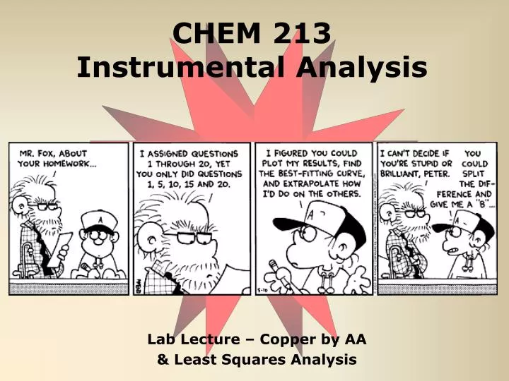
CHEM 213 Instrumental Analysis. Lab Lecture – Copper by AA & Least Squares Analysis. Flame Atomic Absorption. In the gas phase, atomic species will absorb light. General steps: 1. M(ABC) M(XYZ) (aq) M (g) 2. Perform spectroscopy on M (g). Flame AA.

E N D
CHEM 213Instrumental Analysis Lab Lecture – Copper by AA & Least Squares Analysis
Flame Atomic Absorption In the gas phase, atomic species will absorb light. General steps: 1. M(ABC) M(XYZ) (aq) M (g) 2. Perform spectroscopy on M (g)
Flame AA Flame atomizes most molecular species Cu(NO3)2 Cu + NO + NO2 +… Cu in gas phase will absorb light according to Beer’s Law A = aλbc; b = length of flame, c = concentration of vapour in flame Wavelength of absorption depends on the electronic structure of the atomic species (here Cu vapour) Use light source of appropriate wavelength for species being measured. Generate calibration curve and off you go, but…
Normal response Reduced response due to matrix Inst Resp Conc of analyte But… In many methods, the matrix can have significant effects on instrument response. This sample matrix has… Cu, Ni, excess acid, other unknown elements Difficult to reproduce and duplicate Problem: How to account for matrix we cannot reproduce?!?
Calibration by Standard Addition THE method of choice when matrix effects are present/expected 1. Add SAME known volume of unknown (U) to each vial S U 2. Add increasing SMALL volumes of standard (S) to each vial … S0 S1 S2 S3 S4 Volume of standard must be << Volume of sample. Std must be >> concentration of sample
Plotting Std Addition Data Plot CORRECTED Absorbance on Y-Axis [U] = - intercept × [S] / Vol U Get a straight line with X-intercept of – Vol std. added Plot VOLUME of STD Added on X-Axis
General notes: • Prepare stock standard (1.2 to 1.4 mg/mL) and unknown solutions (both in 100 mL). • Pipet 10 mL of unknown into 5×50 mL flasks. • Pipet different amounts of standard to each flask (0, 50, 100, 150, 200 µL). Use 50 µL micropipet • Calibrate the micropipet ahead of time per the instructions on page 46. (The time consuming step) • Record Pipet number and save the pipet tip! • No data printout, so you need to write down all the numbers
Calibration Curves • In 211 used replicate standards of the same concentration to standardize the titrant. • With instruments, response is measured for several concentrations and a calibration curve is developed. • The concentration of an unknown is determined from the curve.
Rules for Calibration curves Unknown must fall within range of standards Y-Axis assumed to contain all error Error independent of magnitude Response Variable X-Axis assumed to be error free Concentration
Graphical Method (plot by hand) • Advantage: By visually inspecting the data, it becomes obvious if the data fall on a line. • Disadvantages: • Line is drawn by “eye” subjective process, imprecise • Difficult to read graph to less than a few parts per thousand. Discard point Use individual measurements Obtain individual concentrations
Method of Least Squares • Advantage: Method is objective and without systematic bias. • Results are usually chosen from this over graphical • Disadvantage: Method is accurate only if the data truly fall on a straight line. • The method itself does not discard points. • Always compare the least squares results with those from the graphical method. • Note: Do NOT simply use the “add trendline” function in Excel. It includes all data points, does not allow for error calculation.
Least Squares Fit Least squares – process of fitting a mathematical function to a set of measured points by minimizing the sum of the squares of the distances from the points to the curve residuals Fig 4-9
Look at your DATA!!! BIG Difference in your result!!!
How does it work? Minimize the sum of the squares of the residuals y = mx + b; yi is measured value, y is predicted value (from equation of line) yi di di = yi - y y
Least Squares Fit • Data points: xi and yi xi = concentration of standard for point i yi = observed response for concentration i • Linear Equation estimate of y: y = mxi + b y residual = yi - (mxi + b), that is yi - y Least Squares Statement: Q =∑[yi - (mxi + b)]2 • find the values of m and b that minimize Q • data that deviates significantly from the line has a large effect on least squares fit
Least Squares Fit • Lab. Manual, page 75-76, Text p 66-67.
Least Squares Fit Lab. Manual, page 77
Drawing a Calibration Curve 1. Manually on graph paper. 2. Mathematically using the least squares method. • Is the calibration curve linear? - can I use y = mx + b ? • What is the best straight line? - what are m and b? • What are the errors in m and b? - what are sm and sb? • What is the error in a determined concentration? - what is sx?
Least Squares Fit y = mx + b deviation = yi - y • Deviation Table Lab. Manual, page 77
Least Squares Fit Errors () in m, b and y (signal) Lab Manual, pg 78
Least Squares Fit Calculation of unknown concentration Lab Manual, pg 78 xunk = (yunk - b)/m • Set up tables to calculate input values for the least-squares equations. • Evaluate b and m. • Evaluate xunk from individual measurements (yiunk) and calculate average. • Evaluate uncertainty in the average value. • Evaluate uncertainty in reported value. -specific to each experiment!!!!
Least Squares Fit Calculation of error in avg unknown concentration Lab Manual, pg 79 k = number of measurements of unknown n = number of points in calibration curve xi = individual x values in calibration curve x = average of all x values in calibration curve y = average of all the y values in the calibration curve y = average of all the values of the y unknown
Least Squares Fit Could also use (easier when doing by hand): k = number of measurements of unknown n = number of points in calibration curve xi = individual x values in calibration curve x = average of all x values FOR UNKNOWN
Chem 213 Least Squares Fit Excel Program Results appear here Enter X values for standards Enter Y values for standards Enter Y values for unknowns Download New_LSQ.xls from www.chem.ualberta.ca/courses/Chem 213/ also available on course website in the Laboratory section
Final Answer Reported • The final answer for the unknown value to be reported most often involves further calculations. • Such calculations will normally require propagation of error calculations to arrive at a final uncertainty. • In particular, note the explicit examples presented in Appendix A of the Laboratory Manual. • Note again the rules for Propagation of Uncertainty and Sig. Fig. Review Chapter 3 of Text!