Download
1 / 25
400 likes | 1k Views
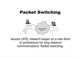
Basic switching concepts circuit switching message switching packet switching. Switching. Circuit Switching Fixed and mobile telephone network Frequency Division Multiplexing (FDM) Time Division Multiplexing (TDM) Optical rings (SDH) Message Switching Not in core technology

E N D
Basic switching conceptscircuit switchingmessage switchingpacket switching
Switching • Circuit Switching • Fixed and mobile telephone network • Frequency Division Multiplexing (FDM) • Time Division Multiplexing (TDM) • Optical rings (SDH) • Message Switching • Not in core technology • Some application (e.g. SMTP) • Packet Switching • Internet • Some core networking technologies (e.g. ATM)
Source rate: 64 kbps 8 bits time 125 ms Link: 64 kbps time Link: 256 kbps time Link: 256 kbps Control information inserted for framing – result: 4x64 > 256! Time Division Multiplexing
switch switch Circuit Switching (i) TDM link TDM slot ctrl … time #1 #2 … #1 #2 … #8 #8 frame Time Division Multiplexing
switch switch Circuit Switching (ii) OUT_A IN_A OUT_B IN_B IN_A OUT_A #1 #2 … #1 #2 … #8 #8 IN_B OUT_B #1 #2 … #1 #2 … #8 #8 IN OUT A,1 B,2 A,3 B,4 SWITCHING TABLE A,4 A,2 Table setup: upon signalling B,1 B,1 B,4 B,3 B,6 A,1 B,7 B,5
Circuit Switching Pros & Cons • Advantages • Limited overhead • Very efficient switching fabrics • Highly parallelized • Disadvantages • Requires signalling for switching tables set-up • Underutilization of resources in the presence of bursty traffic and variable rate traffic Bandwidth waste
Example of bursty traffic(ON/OFF voice flows) On (activity) period OFF period VOICE SOURCE MODEL for conversation (Brady): average ON duration (talkspurt): 1 second average OFF duration (silence): 1,35 seconds Efficiency = utilization % = source activity
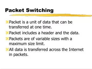
Message vs Packet Switching • Packet Switching • Message chopped in small packets • Each packet includes header • like postal letters! Each must have a specified destination data • Message Switching • One single datagram header message header packet header packet header packet header p Message switching overhead lower than packet switching
Message vs Packet Switching • Packet Switching • Many packets generated by a same node and belonging to a same destination • may take different paths (and packets received out of order – need sequence) • May lose/corrupt a subset (what happens on the message consistency?) • Message Switching • One single datagram • either received or lost • One single network path Message switching: higher reliability, lower complexity header message header packet header packet header packet But sometimes message switching not possible (e.g. for real time sources such as voice) header p
router router Message/packet Switching vs circuit switching • Advantages • Transmission resources used only when needed (data available) • No signalling needed • Disadvantages • Overhead • Inefficient routing fabrics (needs to select output per each packet) • Processing time at routers (routing table lookup) • Queueing at routers Router: - reads header (destination address) - selects output path header mesg/pack
Transmission delay: • C [bit/s] = link rate • B [bit] = packet size • transmission delay = B/C [sec] • Example: • 512 bytes packet • 64 kbps link • transmission delay = 512*8/64000 = 64ms • Propagation delay – constant depending on • Link length • Electromagnetig waves propagation speed in considered media • 200 km/ms for copper links • 300 km/ms in air • other delays neglected • Queueing delay • Processing delay Link delay computation • Delay components: • Processing delay • Transmission delay • Queueing delay • Propagation delay Router sender receiver Tx delay B/C Prop delay Tx delay B/C time time
Router 1 Router 2 Message Switching – delay analysis 320 Kbps 320 Kbps 320 Kbps Tx delay M/C Prop delay Tx delay M/C Prop delay Tx delay M/C time time Example: M=400.000 bytes Header=40 bytes Propagation Tp = 0.050 s Del = 3M/C + 3Tp = 30,153 s Prop delay Tx delay B/C
Router 1 Router 2 Packet Switching – delay analysis 320 Kbps 320 Kbps 320 Kbps Tx delay Mh/C Prop delay Tx delay Ph/C Propdelay Tx delay Ph/C Propdelay time time Packet P = 80000 bytes H = 40 bytes header Ph = 80040 Message: M=400.000 bytes Mh=M+M/P*H=400200 bytes Propagation Tp = 0.050 s Del = Mh/C + 3P + 2Ph/C = 14,157 s Tx delay Mh/C But if packet size = 40 bytes, Del = 20,154s!
Router 3 Router 1 Other example (different link speed) 256 Kbps 256 Kbps 1024 Kbps 2048 Kbps • Time to transmit 1 MB file • Message switching (assume 40 bytes header) • 1MB = 1024*1024 bytes = 1.048.576 bytes = 8.388.608 bits • Including 40 bytes (320 bits) header: 8.388.928 • Neglecting processing, propagation & queueing delays: • D = 32.769 + 8.192 + 4.096 + 32.769 = 77.827s • Packet switching (40 bytes header, 1460 bytes packet) • 718,2 719 packets • total message size including overhead = 8.618.688 • Just considering transmission delays (slowest link = last – try with intermediate, too) • D = 0.047+0.012+0.006 + 33.667 =33.731s • Key advantage: pipelining reduces end to end delay versus message switching!
Statistical Multiplexingthe advantage of packet switching idle idle idle idle Circuit switching: Each slot uniquely Assigned to a flow #1 #2 #3 #4 #1 #2 #3 #4 Full capacity does not imply full utilization!! Packet switching: Each packet grabs The first slot available More flows than nominal capacity may be admitted!!
Overhead for voice sources at 64 Kbps Source rate: 64 kbps 16 ms voice samples = 62,5 samples per sec, each sample = 1024 bit Assumption: 40 bytes header On (activity) period OFF period PACKETIZATION for voice sources (Brady model, activity=42.55%): Assumptions: neglect last packet effect Packet Switching overhead vs burstiness
Packet switching overhead header packet • Header: contains lots of information • Routing, protocol-specific info, etc • Minimum: 28 bytes; in practice much more than 40 bytes • Overhead for every considered protocol: (for voice: 20 bytes IP, 8 bytes UDP, 12 bytes RTP) • Question: how to minimize header while maintaining packet switching? • Solution: label switching (virtual circuit) • ATM • MPLS
switch switch Circuit Switching (again) OUT_A IN_A OUT_B IN_B IN_A OUT_A #1 #2 … #1 #2 … #8 #8 IN_B OUT_B #1 #2 … #1 #2 … #8 #8 IN OUT A,1 B,2 Switching table: route packet coming from Input A, position 1 to output B position 2 A1, B2 = physical slots, can be used onlyby THAT source. Let them be “virtual” (labels on packet!) A,3 B,4 SWITCHING TABLE A,4 A,2 B,1 B,1 B,4 B,3 B,6 A,1 B,7 B,5
switch switch Label Switching (virtual circuit) OUT_A IN_A OUT_B IN_B IN_A OUT_A 10 21 22 61 13 IN_B OUT_B 14 16 19 33 61 12 10 32 87 Condition: labels unique @ input Advantage: labels very small!! (ATM technology overhead: only 5 bytes for all info!) KEY advantage: no reserved phy slots! (asynchronous transfer mode vs synchronous) Label-IN OUT Label-OUT 10 A 61 14 B 61 LABEL SWITCHING TABLE 16 B 12 19 B 87 21 B 10 22 B 32 33 A 13
3 flows Queueuingbuild-up queueuing 2 circuits Statistical mux efficiency(for simplicity, fixed-size packets)
Statistical mux analysis • Very complex, when queueing considered • Involves queueing theory • Involves traffic time correlation statistics High corr Low corr • Very easy, in the (worst case = conservative) assumption of unbuffered system • In practice, burst size long with respect to buffer size • Depends only on activity factor r
Statistical mux analysis (i)unbuffered model N traffic sources; Homogeneous, same activity factor r Source rate = 1; Link capacity = C TDM: N must be <= C Packet: N may be > C Example: N=5; each having 20% activity Average load = 5*0.2 = 1 But C=1 appears insufficient…
Statistical mux analysis (ii)unbuffered model • Overflow probability • Probability that, at a given instant of time (random), the link load is greater than the link capacity • Implies packet loss if buffer=0 Example: N=5; each having 20% activity;
Statistical mux analysis (iii)unbuffered model • Packet loss probability • Number of lost packets over number of offered packets • Offered packets • N * average number of offered packets per source = N * r • Lost packets: • If k <= C active sources, no packet loss • If k > C, k-C lost packets • hence Example: N=5; each having 20% activity; N r = 1
Loss vs overflow Example: N=30; each 20% activity; N r = 6 for C>>Nr: Overflow=good approx for loss.