Download
1 / 53
580 likes | 916 Views
EDGE DETECTION. Edge Detection. Important primitive characteristics of an image: Changes or discontinuities in an image amplitude such as luminance value. Edge and Segment. Local discontinuities in image luminance from one level to another are called luminance edges .

E N D
Edge Detection • Important primitive characteristics of an image: • Changes or discontinuities in an image amplitude such as luminance value
Edge and Segment Local discontinuities in image luminance from one level to another are called luminance edges. Global luminance discontinuities, called luminance boundary segments,
EDGE MODEL • One-dimensional ramp edge modeled as a ramp increase in image amplitude from a low to a high level, or vice versa. • The edge is characterized by its • height, • slope angle, and • horizontal coordinate of the slope midpoint. • An edge exists if the edge height is greater than a specified value. a sketch of a continuous domain
EDGE MODELS • An ideal edge detector: • produce an edge indication localized to a single pixel located at the midpoint of the slope. • If the slope angle of Figure ais 90°, • the resultant edge is called a step edge, • as shown in Figure b. • Step edges usually exist only for artificially generated images
EDGE MODELS • Digital images, resulting from digitization of optical images of real scenes, generally do not possess step edges • Because the anti aliasing low-pass filtering prior to digitization reduces the edge slope in the digital image caused by any sudden luminance change in the scene.
The First-Order Derivative A basic definition of the first-order derivative of a one-dimensional
Second-Order Derivative A second-order derivative as the difference
A Simple Image 1-D horizontal graylevel profile along the center of the image and including the isolated noise point.
Simplified profile (the points are joined by dashed lines to simplify interpretation).
First-order derivatives generally produce thicker edges in an image. • (2) Second-order derivatives have a stronger response to fine detail, such as thin lines and isolated points. • (3) First-order derivatives generally have a stronger response to a gray-level step. • (4) Second-order derivatives produce a double response at step changes in gray level. second-order derivatives: for similar changes in gray-level values in an image, their response is stronger to a line than to a step, and to a point than to a line.
Isotropic filters response is independent of the direction of the discontinuities in the image to which the filter is applied Rotation Invariant rotating the image and then applying the filter gives the same result as applying the filter to the image first and then rotating the result.
FIRST-ORDER DERIVATIVE EDGE DETECTION SCHEMS • There are two fundamental methods for generating first-order derivative edge gradients: • Generation of gradients in two orthogonal directions in an image • Utilizing a set of directional derivatives
Orthogonal Gradient Generation • In the discrete domain, in terms of a row and a column gradient G(j,k):
Orthogonal Gradient Generation For computational efficiency, the gradient amplitude is sometimes approximated by the magnitude combination The orientation of the spatial gradient with respect to the row axis is:
Orthogonal Gradient Generation • Discrete gradient generation is to form the running difference of pixels along rows and columns of the image. The row gradient is defined as The column gradient is
Edeg Detection Operators • Prewitt operator • Roberts Cross-Difference Operator • Sobel Edge Detector • Frei-Chen Operator • Canny Edge Detector • Truncated Pyramid Operator • Argyle and Macleod operator
Prewitt Operator • The separated pixel difference gradient generation method remains highly sensitive to small luminance fluctuations in the image. • Solving: 2-D gradient formation operators that perform • differentiation in one coordinate direction and • spatial averaging in the orthogonal direction simultaneously.
Prewitt operator • Prewitt has introduced a 3x3 pixel edge gradient operator. • The Prewitt operator square root edge gradient is defined as:
Prewitt Operators The row and column gradients for all the edge detectors involve a linear combination of pixels within a small neighborhood. The row and column gradients can be computed by the convolution relationships: row and column impulse response arrays
Prewitt Operators • A limitation common to the edge gradient generation operators is their inability to detect accurately edges in high-noise environments. • This problem can be alleviated by properly extending the size of the neighborhood operators over which the differential gradients are computed.
Prewitt Operators • A Prewitt type 7x7 operator has a row gradient impulse response of the form An operator of this type is called a boxcar operator
Roberts Cross Edge Detector • Performs a simple, quick to compute, 2-D spatial gradient measurement on an image. • It highlights regions of high spatial frequency which often correspond to edges. • In its most common usage, • the input a grayscale image, as is the output. • Output pixel values at each point represent the estimated absolute magnitude of the spatial gradient at that point.
How Roberts Cross Edge Detector Works • The operator consists of a pair of 2×2 convolution kernels as shown below One kernel is the other rotated by 90°
How Roberts Cross Edge Detector Works • Kernels are designed to respond maximally to edges running at 45° to the pixel grid, one kernel for each of the two perpendicular orientations. • Kernels can be applied separately to the input image, to produce separate measurements of the gradient component in each orientation (Gx and Gy). • These can be combined together to find the absolute magnitude of the gradient at each point and the orientation of that gradient.
The gradient magnitude is given by: The angle of orientation of the edge giving rise to the spatial gradient (relative to the pixel grid orientation) is given by:
Often, the absolute magnitude is the only output the user sees. The two components of the gradient are computed and added in a single pass using the pseudo-convolution operator shown below.
The main reason for using the Roberts Cross operator is that it is very quick to compute. Only four input pixels need to be examined to determine the value of each output pixel. 1. Only subtractions and additions are used . 2. There are no parameters to set. Disadvantage High noise sensitivity
The result of thresholding output at a pixel value of 80 The spurious bright dots on the image which demonstrate that the operator is susceptible to noise Only the strongest edges have been detected with any reliability
Example Roberts Cross operator Edge detection Threshold the image at a value of 20, all depth discontinuities in the object produce an edge in the image
Noise Sensitivity Threshold the image at a value of 20 Output of the Roberts Cross operator
Noise Sensitivity range image where the depth values change much more slowly The edges in the resulting Roberts Cross image are rather faint Thresholding the image at a value of 30 Since the intensity of many edge pixels in this image is very low, it is not possible to entirely separate the edges from the noise
The effects of the shape of the edge detection kernel on the edge image Due to the different width and orientation of the lines in the image, the response in the edge image varies significantly. The intensity steps between foreground and background are constant in all patterns of the original image, This shows that : the Roberts Cross operator responds differently to different frequencies and orientations.
Sobel Edge Detector The Sobel operator performs a 2-D spatial gradient measurement on an image and so emphasizes regions of high spatial frequency that correspond to edges. Typically it is used to find the approximate absolute gradient magnitude at each point in an input grayscale image.
How Sobel Operator Works The operator consists of a pair of 3×3 convolution kernels as shown below. One kernel is simply the other rotated by 90°. This is very similar to the Roberts Cross operator.
These kernels are designed to respond maximally to edges running vertically and horizontally relative to the pixel grid. One kernel for each of the two perpendicular orientations. The kernels can be applied separately to the input image, to produce separate measurements of the gradient component in each orientation (Gx and Gy). These can then be combined together to find the absolute magnitude of the gradient at each point and the orientation of that gradient.
The gradient magnitude is given by: An approximate magnitude is computed using: The angle of orientation of the edge (relative to the pixel grid) giving rise to the spatial gradient is given by: Orientation 0 is taken to mean that the direction of maximum contrast from black to white runs from left to right on the image, and other angles are measured anti-clockwise from this.
The absolute magnitude is the only output the user sees. The two components of the gradient are computed and added in a single pass over the input image. The pseudo-convolution operator shown in Figure below is employed.
Sobel Edge Detector Specifications 1. The Sobel operator is slower to compute than the Roberts Cross operator. 2. Its larger convolution kernel smooths the input image to a greater extent makes the operator less sensitive to noise. 3. The operator produces higher output values for similar edges, compared with the Roberts Cross.
Sobel Edge Detector Specifications Natural edges often lead to lines that are several pixels widedue to the smoothing effect of the Sobel operator. Some thinning may be desirable to counter this.
Sobel Edge Detector Specifications Roberts Cross Sobel operator The spurious noise that afflicted the Roberts Cross output image is still present, but its intensity relative to the genuine lines has been reduced, we may get rid of this entirely by thresholding. The lines corresponding to edges have become thicker compared with the Roberts Cross output due to the increased smoothing of the Sobel operator.
Sobel Edge Detector Specifications All edges have been detected and can be separated from the background using a threshold value (150)
The Sobel operator is not as sensitive to noise as the Roberts Cross operator, it still amplifies high frequencies. The noise has increased during the edge detection. It is no longer possible to find a threshold which removes all noise pixels and at the same time retains the edges of the objects
Sobel Edge Detector Specifications The object in the previous example contains: sharp edges and its surface is rather smooth. we could (in the noise-free case) easily detect the boundary of the object without getting any erroneous pixels. A more difficult task is to detect the boundary of:
The intensity of many pixels on the surface is as high as along the actual edges. One reason is that the output of many edge pixels is greater than the maximum pixel value and therefore they are `cut off' at 255. To avoid this overflow we scale the range image by a factor 0.25 prior to the edge detection and then normalize the output