Download
1 / 14
150 likes | 314 Views
Application of HMMs: Speech recognition. “Noisy channel” model of speech. Speech feature extraction. Acoustic wave form Sampled at 8KHz, quantized to 8-12 bits. Amplitude. Spectrogram. Frequency. Time. Frame (10 ms or 80 samples). Feature vector ~39 dim. Speech feature extraction.

E N D
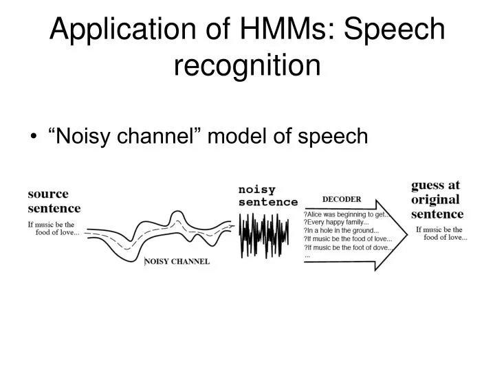
Application of HMMs: Speech recognition • “Noisy channel” model of speech
Speech feature extraction Acoustic wave form Sampled at 8KHz, quantized to 8-12 bits Amplitude Spectrogram Frequency Time Frame (10 ms or 80 samples) Feature vector ~39 dim.
Speech feature extraction Acoustic wave form Sampled at 8KHz, quantized to 8-12 bits Amplitude Spectrogram Frequency Time Frame (10 ms or 80 samples) Feature vector ~39 dim.
Phonetic model • Phones: speech sounds • Phonemes: groups of speech sounds that have a unique meaning/function in a language (e.g., there are several different ways to pronounce “t”)
HMM models for phones • HMM states in most speech recognition systems correspond to subphones • There are around 60 phones and as many as 603 context-dependent triphones
Putting words together • Given a sequence of acoustic features, how do we find the corresponding word sequence?
Limitations of Viterbi decoding • Number of states may be too large • Beam search: at each time step, maintain a short list of the most probable words and only extend transitions from those words into the next time step • Words with multiple pronunciation variants may get a smaller probability than incorrect words with fewer pronunciation paths Word model for “tomato”
Limitations of Viterbi decoding • Number of states may be too large • Beam search: at each time step, maintain a short list of the most probable words and only extend transitions from those words into the next time step • Words with multiple pronunciation variants may get a smaller probability than incorrect words with fewer pronunciation paths • Use the forward algorithm instead of Viterbi algorithm • The Markov assumption is too weak to capture the constraints of real language
Advanced techniques • Multiple pass decoding • Let the Viterbi decoder return multiple candidate utterances and then re-rank them using a more sophisticated language model, e.g., n-gram model
Advanced techniques • Multiple pass decoding • Let the Viterbi decoder return multiple candidate utterances and then re-rank them using a more sophisticated language model, e.g., n-gram model • A* decoding • Build a search tree whose nodes are words and whose paths are possible utterances • Path cost is given by the likelihood of the acoustic features given the words inferred so far • Heuristic function estimates the best-scoring extension until the end of the utterance
Reference • D. Jurafsky and J. Martin, “Speech and Language Processing,” 2nd ed., Prentice Hall, 2008