Download
1 / 50
500 likes | 638 Views
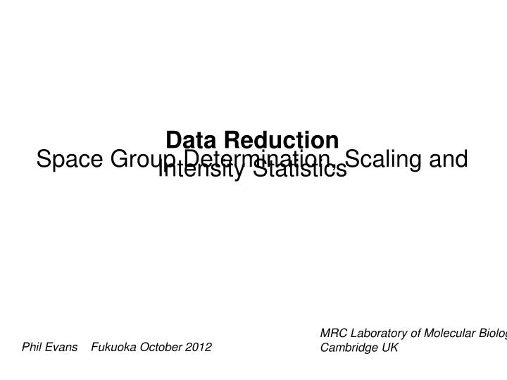
Data Reduction Space Group Determination, Scaling and Intensity Statistics. MRC Laboratory of Molecular Biology Cambridge UK. Phil Evans Fukuoka October 2012. Intensities from eg Mosflm, XDS etc h k l I σ(I) etc. h k l F σ(F) I σ(I) FreeR_flag. Scaling and Merging. Experiment.

E N D
Data ReductionSpace Group Determination, Scaling and Intensity Statistics MRC Laboratory of Molecular Biology Cambridge UK Phil Evans Fukuoka October 2012
Intensities from eg Mosflm, XDS etc h k l I σ(I) etc h k l F σ(F) I σ(I) FreeR_flag Scaling and Merging Experiment |F|2 I lots of effects (“errors”) Our job is to invert the experiment: we want to infer |F| from our measurements of intensity I Model of experiment I |F|2 |F| Parameterise experiment
Integration and data reduction can be done in an automated pipeline such as XIA2 (Graeme Winter): this goes from images to a list of hkl F ready for structure determination) Automation works pretty well, but in difficult cases you may need finer control over the process
Intensities from Mosflm (or XDS) h k l I σ(I) etc Intensities from Mosflm (or XDS) h k l I σ(I) etc Intensities from Mosflm (or XDS) h k l I σ(I) etc UNIQUIFY etc CTRUNCATE AIMLESS/SCALA POINTLESS h k l F σ(F) I σ(I) FreeR_flag Scaled and averaged intensities Sorted Intensities in “best” space group Data flow scheme in CCP4 Note that multiple files from different “sweeps” or crystals can be combined One or more files from integration program One or more datasets (eg MAD) Complete sphere of reflections Generate or copy freeR flags Determine point-group (& space group) and consistent indexing Estimate |F| from I detect twinning (intensity statistics) Scale symmetry-related intensities together Produce statistics on data quality These programs may ultimately be combined into one
Track one reflection through the process Spot over 4 images 3D integration eg XDS, d*trek 7 6 5 4 2D integration eg Mosflm, hkl2000 In MTZ file from Mosflm, ordered by image (BATCH) number Entries spread through file Spot profile h k l M/ISYM BATCH I SIGI IPR SIGIPR ... -20 12 10 258 4 13 3 7 3... -20 12 10 258 5 304 24 322 24... -20 12 10 258 6 1072 84 1101 84... -20 12 10 258 7 349 27 324 27 After POINTLESS: Possibly reindexed observation parts grouped by reduced hkl (sorted) Profile fit Summation integration Full/part+ Symmetry number Image number Partial serial Detector pixel Reduced hkl Original hkl Width Intensities & σ(I) Fraction Rotation LP Flags Symmetry-related observations
CTRUNCATE AIMLESS Unmerged file from Pointless, multiple entries for each unique hkl (note that we need to know the point group to connect these) Full Partial Three symmetry-related observations for one reflection Partial scale and merge Merged file, one line for each hkl Optional unmerged output Partials summed, scaled, outliers rejected Infer |F| from I Merged file, one line for each hkl, intensities and amplitudes F
Determination of Space group The space group symmetry is only a hypothesis until the structure is solved, since it is hard to distinguish between true crystallographic and approximate (non-crystallographic) symmetry. By examining the symmetry of the diffraction pattern we can get a good idea of the likely space group It is also useful to find the likely symmetry as early as possible, since this affects the data collection strategy Stage 1: lattice symmetry From the unit cell dimensions we can deduce the maximum possible lattice symmetry, ie the crystal system: this the only information available to the integration program (Mosflm) Systems are : cubic, hexagonal/trigonal, tetragonal, orthorhombic, monoclinic, or triclinic, + lattice centring P, C, I, R, or F For example if a = b = c and α=β=γ=90° (within some tolerance eg 2°) then the maximum lattice symmetry is cubic
Analysing rotational symmetry in lattice group P m -3 m----------------------------------------------Scores for each symmetry elementNelmt Lklhd Z-cc CC N Rmeas Symmetry & operator (in Lattice Cell) 1 0.955 9.70 0.97 13557 0.073 identity 2 0.062 2.66 0.27 12829 0.488 2-fold ( 1 0 1) {+l,-k,+h} 3 0.065 2.85 0.29 10503 0.474 2-fold ( 1 0-1) {-l,-k,-h} 4 0.056 0.06 0.01 16391 0.736 2-fold ( 0 1-1) {-h,-l,-k} 5 0.057 0.05 0.00 17291 0.738 2-fold ( 0 1 1) {-h,+l,+k} 6 0.049 0.55 0.06 13758 0.692 2-fold ( 1-1 0) {-k,-h,-l} 7 0.950 9.59 0.96 12584 0.100 *** 2-fold k ( 0 1 0) {-h,+k,-l} 8 0.049 0.57 0.06 11912 0.695 2-fold ( 1 1 0) {+k,+h,-l} 9 0.948 9.57 0.96 16928 0.136 *** 2-fold h ( 1 0 0) {+h,-k,-l} 10 0.944 9.50 0.95 12884 0.161 *** 2-fold l ( 0 0 1) {-h,-k,+l} 11 0.054 0.15 0.01 23843 0.812 3-fold ( 1 1 1) {+l,+h,+k} {+k,+l,+h} 12 0.055 0.11 0.01 24859 0.825 3-fold ( 1-1-1) {-l,-h,+k} {-k,+l,-h} 13 0.055 0.14 0.01 22467 0.788 3-fold ( 1-1 1) {+l,-h,-k} {-k,-l,+h} 14 0.055 0.12 0.01 27122 0.817 3-fold ( 1 1-1) {-l,+h,-k} {+k,-l,-h} 15 0.061 -0.10 -0.01 25905 0.726 4-fold h ( 1 0 0) {+h,-l,+k} {+h,+l,-k} 16 0.060 2.53 0.25 23689 0.449 4-fold k ( 0 1 0) {+l,+k,-h} {-l,+k,+h} 17 0.049 0.56 0.06 25549 0.653 4-fold l ( 0 0 1) {-k,+h,+l} {+k,-h,+l} Stage 2: individual rotational symmetry operators Ignore symmetry from integration program Test all rotation operators consistent with the lattice symmetry Score agreement between reflections related by each operator, by R-factor (Rmeas) and correlation coefficient (CC) on normalised intensities |E|2 Calculate a “probability” based on the CC Pseudo-cubic example Cell: 79.15 81.33 81.15 90.00 90.00 90.00 a ≈ b ≈ c Only orthorhombic symmetry operators are present
CC = 0.06 CC = 0.94 What score to use? Linear correlation coefficient For equal axes, the correlation coefficient (CC) is the slope of the “best” (least-squares) straight line through the scatter plot CCs have the advantage over eg R-factors in being relatively insensitive to incorrect scales ... but they are more sensitive to outliers ... and CCs need to correlate values that come from the same distribution, ie in this case |E|2 rather than I
Stage 3: point group All possible combinations of rotations are scored to determine the point group. Good scores in symmetry operations which are absent in the sub-group count against that group. Example: C-centred orthorhombic which might been hexagonal Laue Group Lklhd NetZc Zc+ Zc- CC CC- Rmeas R- Delta ReindexOperator= 1 C m m m *** 0.989 9.45 9.62 0.17 0.96 0.02 0.08 0.76 0.0 [h,k,l] 2 P 1 2/m 1 0.004 7.22 9.68 2.46 0.97 0.25 0.06 0.56 0.0 [-1/2h+1/2k,-l,-1/2h-1/2k] 3 C 1 2/m 1 0.003 7.11 9.61 2.50 0.96 0.25 0.08 0.55 0.0 [h,k,l] 4 C 1 2/m 1 0.003 7.11 9.61 2.50 0.96 0.25 0.08 0.55 0.0 [-k,-h,-l] 5 P -1 0.000 6.40 9.67 3.27 0.97 0.33 0.06 0.49 0.0 [1/2h+1/2k,1/2h-1/2k,-l] 6 C m m m 0.000 1.91 5.11 3.20 0.51 0.32 0.34 0.51 2.5 [1/2h-1/2k,-3/2h-1/2k,-l] 7 P 6/m 0.000 1.16 4.59 3.43 0.46 0.34 0.41 0.46 2.5 [-1/2h-1/2k,-1/2h+1/2k,-l] 8 C 1 2/m 1 0.000 1.51 5.15 3.64 0.52 0.36 0.33 0.47 2.5 [1/2h-1/2k,-3/2h-1/2k,-l] 9 C 1 2/m 1 0.000 1.51 5.15 3.64 0.51 0.36 0.33 0.47 2.5 [-3/2h-1/2k,-1/2h+1/2k,-l] 10 P -3 0.000 1.04 4.75 3.71 0.48 0.37 0.40 0.45 2.5 [-1/2h-1/2k,-1/2h+1/2k,-l] 11 C m m m 0.000 2.13 5.23 3.10 0.52 0.31 0.32 0.52 2.5 [-1/2h-1/2k,-3/2h+1/2k,-l] 12 C 1 2/m 1 0.000 1.64 5.25 3.61 0.53 0.36 0.32 0.47 2.5 [-1/2h-1/2k,-3/2h+1/2k,-l] 13 C 1 2/m 1 0.000 1.67 5.27 3.60 0.53 0.36 0.32 0.47 2.5 [-3/2h+1/2k,1/2h+1/2k,-l] 14 P -3 1 m 0.000 0.12 4.00 3.87 0.40 0.39 0.44 0.44 2.5 [-1/2h-1/2k,-1/2h+1/2k,-l] 15 P -3 m 1 0.000 0.14 4.00 3.86 0.40 0.39 0.44 0.44 2.5 [-1/2h-1/2k,-1/2h+1/2k,-l] 16 P 6/m m m 0.000 3.93 3.93 0.00 0.39 0.00 0.44 0.00 2.5 [-1/2h-1/2k,-1/2h+1/2k,-l]
Analysing rotational symmetry in lattice group P 6/m m m----------------------------------------------Scores for each symmetry elementNelmt Lklhd Z-cc CC N Rmeas Symmetry & operator (in Lattice Cell) 1 0.932 9.94 0.99 1299 0.033 identity 2 0.794 8.19 0.82 1328 0.168 ** 2-fold l ( 0 0 1) {-h,-k,l} 3 0.815 8.29 0.83 1346 0.168 ** 2-fold k ( 0 1 0) {-h,h+k,-l} 4 0.625 7.55 0.76 1340 0.171 * 2-fold h ( 1 0 0) {h+k,-k,-l} 5 0.653 7.65 0.77 1362 0.173 * 2-fold ( 1-1 0) {-k,-h,-l} 6 0.934 9.83 0.98 1510 0.048 *** 2-fold ( 2-1 0) {h,-h-k,-l} 7 0.934 9.85 0.99 1486 0.045 *** 2-fold (-1 2 0) {-h-k,k,-l} 8 0.936 9.72 0.97 1450 0.055 *** 2-fold ( 1 1 0) {k,h,-l} 9 0.936 9.66 0.97 3007 0.065 *** 3-fold l ( 0 0 1) {k,-h-k,l}{-h-k,h,l} 10 0.503 7.09 0.71 2790 0.186 * 6-fold l ( 0 0 1) {h+k,-h,l}{-k,h+k,l} What can go wrong? A bad case Pseudo-symmetry or twinning (often connected) can suggest a point group symmetry which is too high Careful examination of the scores for individual symmetry operators may indicate the truth (the program is not foolproof!) Twinning not detected by L-test though probably present Correct operators indicated for 321 point group
What can go wrong? Pseudo-symmetry or twinning (often connected) can suggest a point group symmetry which is too high Careful examination of the scores for individual symmetry operators may indicate the truth (the program is not foolproof!) ... but POINTLESS selects the wrong Laue group in this case Laue Group Lklhd NetZc Zc+ Zc- CC CC- Rmeas R- Delta ReindexOperator= 1 P 6/m m m *** 0.981 8.74 8.74 0.00 0.87 0.00 0.11 0.00 0.0 [h,k,l] 2 P -3 m 1 0.018 2.10 9.80 7.70 0.98 0.77 0.05 0.17 0.0 [h,k,l] 3 C m m m 0.000 0.60 9.10 8.50 0.91 0.85 0.10 0.11 0.0 [h,h+2k,l] 4 P -3 1 m 0.000 -0.12 8.68 8.80 0.87 0.88 0.11 0.10 0.0 [h,k,l] 5 C m m m 0.000 0.29 8.92 8.62 0.89 0.86 0.10 0.11 0.0 [h+k,-h+k,l] 6 C m m m 0.000 0.33 8.94 8.61 0.89 0.86 0.10 0.11 0.0 [-k,2h+k,l] 7 P 6/m 0.000 -0.09 8.69 8.78 0.87 0.88 0.11 0.11 0.0 [h,k,l] 8 P -3 0.000 1.38 9.81 8.43 0.98 0.84 0.05 0.13 0.0 [h,k,l] 9 C 1 2/m 1 0.000 1.39 9.84 8.45 0.98 0.84 0.04 0.13 0.0 [h-k,h+k,l] 10 C 1 2/m 1 0.000 1.45 9.89 8.44 0.99 0.84 0.04 0.13 0.0 [h+2k,-h,l] 11 C 1 2/m 1 0.000 1.48 9.90 8.43 0.99 0.84 0.04 0.13 0.0 [2h+k,k,l] 12 C 1 2/m 1 0.000 0.60 9.21 8.61 0.92 0.86 0.09 0.11 0.0 [h,h+2k,l] 13 P 1 2/m 1 0.000 0.55 9.17 8.62 0.92 0.86 0.09 0.11 0.0 [k,l,h] 14 C 1 2/m 1 0.000 0.20 8.90 8.70 0.89 0.87 0.09 0.11 0.0 [h+k,-h+k,l] 15 C 1 2/m 1 0.000 0.16 8.86 8.70 0.89 0.87 0.09 0.11 0.0 [-k,2h+k,l] 16 P -1 0.000 1.37 9.94 8.58 0.99 0.86 0.03 0.12 0.0 [l,-h,-k]
Stage 4: space group from axial systematic absences Fourier analysis of I/σ(I) There are indications of 21 screw symmetry along all principle axes (though note there are only 3 observations on the a axis (h00 reflections)) Possible 21 axis along a Clear 21 axis along b Clear 21 axis along c ... BUT “confidence” in space group may be low due to sparse or missing information Always check the space group later in the structure solution!
Note high confidence in Laue group, but lower confidence in space group
Analysing rotational symmetry in lattice group P m -3 m----------------------------------------------Scores for each symmetry elementNelmt Lklhd Z-cc CC N Rmeas Symmetry & operator (in Lattice Cell) 1 0.955 9.70 0.97 13557 0.073 identity 2 0.062 2.66 0.27 12829 0.488 2-fold ( 1 0 1) {+l,-k,+h} 3 0.065 2.85 0.29 10503 0.474 2-fold ( 1 0-1) {-l,-k,-h} 4 0.056 0.06 0.01 16391 0.736 2-fold ( 0 1-1) {-h,-l,-k} 5 0.057 0.05 0.00 17291 0.738 2-fold ( 0 1 1) {-h,+l,+k} 6 0.049 0.55 0.06 13758 0.692 2-fold ( 1-1 0) {-k,-h,-l} 7 0.950 9.59 0.96 12584 0.100 *** 2-fold k ( 0 1 0) {-h,+k,-l} 8 0.049 0.57 0.06 11912 0.695 2-fold ( 1 1 0) {+k,+h,-l} 9 0.948 9.57 0.96 16928 0.136 *** 2-fold h ( 1 0 0) {+h,-k,-l} 10 0.944 9.50 0.95 12884 0.161 *** 2-fold l ( 0 0 1) {-h,-k,+l} 11 0.054 0.15 0.01 23843 0.812 3-fold ( 1 1 1) {+l,+h,+k} {+k,+l,+h} 12 0.055 0.11 0.01 24859 0.825 3-fold ( 1-1-1) {-l,-h,+k} {-k,+l,-h} 13 0.055 0.14 0.01 22467 0.788 3-fold ( 1-1 1) {+l,-h,-k} {-k,-l,+h} 14 0.055 0.12 0.01 27122 0.817 3-fold ( 1 1-1) {-l,+h,-k} {+k,-l,-h} 15 0.061 -0.10 -0.01 25905 0.726 4-fold h ( 1 0 0) {+h,-l,+k} {+h,+l,-k} 16 0.060 2.53 0.25 23689 0.449 4-fold k ( 0 1 0) {+l,+k,-h} {-l,+k,+h} 17 0.049 0.56 0.06 25549 0.653 4-fold l ( 0 0 1) {-k,+h,+l} {+k,-h,+l} Laue Group Lklhd NetZc Zc+ Zc- CC CC- Rmeas R- Delta ReindexOperator= 1 P m m m *** 0.989 8.93 9.59 0.66 0.96 0.07 0.12 0.69 0.0 [-h,-l,-k] 2 P 1 2/m 1 0.003 7.85 9.65 1.80 0.97 0.18 0.09 0.60 0.0 [-h,-l,-k] 3 P 1 2/m 1 0.003 7.95 9.63 1.68 0.96 0.17 0.10 0.61 0.0 [l,h,k] 4 P 1 2/m 1 0.003 7.80 9.61 1.81 0.96 0.18 0.11 0.60 0.0 [h,k,l] 5 P 4/m m m 0.000 6.69 6.90 0.21 0.69 0.02 0.24 0.75 1.5 [-k,-h,-l] 6 P 4/m m m 0.000 4.55 5.41 0.85 0.54 0.09 0.34 0.68 0.1 [-l,-k,-h] 7 P 4/m 0.000 5.45 7.20 1.75 0.72 0.18 0.20 0.62 1.5 [-k,-h,-l] 8 P 4/m 0.000 4.72 6.53 1.81 0.65 0.18 0.25 0.60 0.1 [-l,-k,-h] 9 P -1 0.000 7.48 9.70 2.22 0.97 0.22 0.07 0.57 0.0 [-h,-l,-k] 10 P 4/m 0.000 4.03 5.96 1.92 0.60 0.19 0.29 0.59 1.4 [-h,-l,-k] 11 P 4/m m m 0.000 4.93 5.63 0.69 0.56 0.07 0.32 0.69 1.4 [-h,-l,-k] 12 C m m m 0.000 4.97 6.67 1.70 0.67 0.17 0.24 0.62 1.5 [h-k,-h-k,-l] 13 C 1 2/m 1 0.000 4.80 6.99 2.19 0.70 0.22 0.21 0.57 1.5 [-h-k,-h+k,-l] 14 C 1 2/m 1 0.000 4.51 6.71 2.20 0.67 0.22 0.23 0.58 1.5 [h-k,-h-k,-l] 15 C m m m 0.000 3.08 5.01 1.93 0.50 0.19 0.36 0.59 0.1 [-k-l,-k+l,-h] 16 P m -3 0.000 3.35 4.32 0.97 0.43 0.10 0.44 0.63 1.5 [h,k,l] 17 C 1 2/m 1 0.000 2.58 4.95 2.36 0.49 0.24 0.35 0.56 0.1 [k-l,-k-l,-h] 18 C 1 2/m 1 0.000 2.65 5.01 2.36 0.50 0.24 0.34 0.56 0.1 [-k-l,-k+l,-h] 19 H -3 0.000 2.17 4.56 2.39 0.46 0.24 0.40 0.55 1.5 [-k+l,-h-l,h-k-l] 20 H -3 0.000 2.09 4.48 2.39 0.45 0.24 0.40 0.55 1.5 [h-l,-h-k,-h+k-l] 21 H -3 0.000 2.15 4.54 2.39 0.45 0.24 0.39 0.55 1.5 [-h+k,-k-l,-h-k+l] 22 H -3 0.000 2.20 4.59 2.38 0.46 0.24 0.39 0.55 1.5 [k-l,h-k,-h-k-l] 23 C 1 2/m 1 0.000 3.10 5.42 2.32 0.54 0.23 0.31 0.56 1.4 [-h-l,h-l,-k] 24 C 1 2/m 1 0.000 3.36 5.67 2.31 0.57 0.23 0.30 0.56 1.4 [-h+l,-h-l,-k] 25 C m m m 0.000 3.32 5.29 1.97 0.53 0.20 0.34 0.59 1.4 [-h-l,h-l,-k] 26 H -3 m 0.000 -0.01 2.66 2.67 0.27 0.27 0.52 0.54 1.5 [-h+k,-k-l,-h-k+l] 27 H -3 m 0.000 -0.03 2.65 2.68 0.26 0.27 0.52 0.54 1.5 [k-l,h-k,-h-k-l] 28 H -3 m 0.000 -0.13 2.58 2.71 0.26 0.27 0.53 0.53 1.5 [h-l,-h-k,-h+k-l] 29 H -3 m 0.000 -0.02 2.66 2.68 0.27 0.27 0.52 0.53 1.5 [-k+l,-h-l,h-k-l] 30 P m -3 m 0.000 2.67 2.67 0.00 0.27 0.00 0.53 0.00 1.5 [h,k,l] Only orthorhombic symmetry operators are present ... symmetry is actually orthorhombic (P 21 21 21) Pseudo-cubic example Cell: 79.15 81.33 81.15 90.00 90.00 90.00 a ≈ b ≈ c
Dataset 1, pk, 3 files 3 files assigned to same dataset Dataset 2, ip, 1 file Dataset 3, rm, 1 file Because of an indexing ambiguity (pseudo-cubic orthorhombic), we must check for consistent indexing between files Combining multiple files (and multiple MAD datasets)
Space group from HKLIN file : R 3 :H Cell: 257.89 257.89 144.72 90.00 90.00 120.00Alternative index test relative to reference file Alternative reindexing CC R(E^2) Number Cell_deviation [h,k,l] 0.885 0.157 6537 0.81 [k,h,-l] -0.001 0.511 6084 0.81 Alternative indexing If the true point group is lower symmetry than the lattice group, alternative valid but non-equivalent indexing schemes are possible, related by symmetry operators present in lattice group but not in point group (note that these are also the cases where merohedral twinning is possible) eg if in space group P3 (or P31) there are 4 different schemes (h,k,l) or (-h,-k,l) or (k,h,-l) or (-k,-h,-l) For the first crystal, you can choose any scheme For subsequent crystals, the autoindexing will randomly choose one setting, and we need to make it consistent: POINTLESS will do this for you by comparing the unmerged test data to a reference dataset (merged or unmerged)
A confusing case in C222: Unit cell 74.72 129.22 184.25 90 90 90 This has b ≈ √3 a so can also be indexed on a hexagonal lattice, lattice point group P622 (P6/mmm), with the reindex operator: h/2+k/2, h/2-k/2, -l Conversely, a hexagonal lattice may be indexed as C222 in three distinct ways, so there is a 2 in 3 chance of the indexing program choosing the wrong one Hexagonal axes (black) Three alternative C-centred orthorhombic Lattices (coloured)
Rfactor (multiplicity weighted) “Likelihood” Correlation coefficient on E2 Z-score(CC) Nelmt Lklhd Z-cc CC N Rmeas Symmetry & operator (in Lattice Cell) 1 0.808 5.94 0.89 9313 0.115 identity 2 0.828 6.05 0.91 14088 0.141 *** 2-fold l ( 0 0 1) {-h,-k,+l} 3 0.000 0.06 0.01 16864 0.527 2-fold ( 1-1 0) {-k,-h,-l} 4 0.871 6.33 0.95 10418 0.100 *** 2-fold ( 2-1 0) {+h,-h-k,-l} 5 0.000 0.53 0.08 12639 0.559 2-fold h ( 1 0 0) {+h+k,-k,-l} 6 0.000 0.06 0.01 16015 0.562 2-fold ( 1 1 0) {+k,+h,-l} 7 0.870 6.32 0.95 2187 0.087 *** 2-fold k ( 0 1 0) {-h,+h+k,-l} 8 0.000 0.55 0.08 7552 0.540 2-fold (-1 2 0) {-h-k,+k,-l} 9 0.000 -0.12 -0.02 11978 0.598 3-fold l ( 0 0 1) {-h-k,+h,+l} {+k,-h-k,+l} 10 0.000 -0.06 -0.01 17036 0.582 6-fold l ( 0 0 1) {-k,+h+k,+l} {+h+k,-h,+l} Score each symmetry operator in P622 Only the orthorhombic symmetry operators are present
Intensities from Mosflm (or XDS) h k l I σ(I) etc Intensities from Mosflm (or XDS) h k l I σ(I) etc Intensities from Mosflm (or XDS) h k l I σ(I) etc UNIQUIFY etc CTRUNCATE AIMLESS/SCALA POINTLESS h k l F σ(F) I σ(I) FreeR_flag Scaled and averaged intensities Sorted Intensities in “best” space group Data flow scheme in CCP4 One or more files from integration program One or more datasets (eg MAD) Note that this does not work well for very large numbers of crystals Complete sphere of reflections Generate or copy freeR flags Determine point-group (& space group) and consistent indexing Estimate |F| from I detect twinning (intensity statistics) Scale symmetry-related intensities together Produce statistics on data quality These programs may ultimately be combined into one
Choices • What scaling model? • the scaling model should reflect the experiment considerations of scaling may affect design of experiment • Is the dataset any good? • should it be thrown away immediately? • what is the real resolution? • are there bits which should be discarded (bad images)?
Why are reflections on different scales? Various physical factors lead to observed intensities being on different scales. Some corrections are known eg Lorentz and polarisation corrections, but others can only be determined from the data Scaling models should if possible parameterise the experiment so different experiments may require different models Understanding the effect of these factors allows a sensible design of correction and an understanding of what can go wrong (a) Factors related to incident beam and the camera (b) Factors related to the crystal and the diffracted beam (c) Factors related to the detector
Factors related to incident Xray beam (a) incident beam intensity: variable on synchrotrons and not normally measured. Assumed to be constant during a single image, or at least varying smoothly and slowly (relative to exposure time). If this is not true, the data will be poor (b) illuminated volume: changes with φ if beam smaller than crystal (c) absorption in primary beam by crystal: indistinguishable from (b) (d) variations in rotation speed and shutter synchronisation. These errors are disastrous, difficult to detect, and (almost) impossible to correct for: we assume that the crystal rotation rate is constant and that adjacent images exactly abut in φ. (Shutter synchronisation errors lead to partial bias which may be positive, unlike the usual negative bias) Data collection with open shutter (eg with Pilatus detector) avoids synchronisation errors (though variation in rotation speed could still cause trouble, and there is a dead time during readout)
Factors related to crystal and diffracted beam (e) Absorption in secondary beam - serious at long wavelength (including CuKα) (f) radiation damage - serious on high brilliance sources. Not easily correctable unless small as the structure is changing Maybe extrapolate back to zero time? (but this needs high multiplicity) The relative B-factor is largely a correction for the average radiation damage
Factors related to the detector • The detector should be properly calibrated for spatial distortion and sensitivity of response, and should be stable. Problems with this are difficult to detect from diffraction data. There are known problems in the tile corners of CCD detectors (corrected for in XDS) • The useful area of the detector should be calibrated or told to the integration program – Calibration should flag defective pixels (hot or cold) and dead regions eg between tiles – The user should tell the integration program about shadows from the beamstop, beamstop support or cryocooler (define bad areas by circles, rectangles, arcs etc)
Scaling Scaling tries to make symmetry-related and duplicate measurements of a reflection equal, by modelling the diffraction experiment, principally as a function of the incident and diffracted beam directions in the crystal. This makes the data internally consistent. Note that we do not know the true intensities and an internally-consistent dataset is not necessarily correct. Systematic errors which are the same for symmetry-related reflections will remain Minimize Φ = Σhl whl (Ihl - 1/khl<Ih>)2 Ihl l’th intensity observation of reflection h khl scale factor for Ihl<Ih> current estimate of Ih ghl = 1/khl is a function of the parameters of the scaling model ghl = g(φ rotation/image number) . g(time) . g(s) ...other factors Primary beam s0 B-factor Absorption
How can we measure data quality? After scaling, the remaining differences between symmetry-related observations can be analysed to give an indication of data quality, though not necessarily of its absolute correctness. We can also compare the intensities with their estimated errors to get signal/noise ratio A. Measures of statistical significance: I/σ(I) after averaging symmetry-related observations and after “correcting” σ(I) estimates (“Mn(I/sd)” in AIMLESS and SCALA output) is a measure of signal/noise – but is sensitive to problems in the estimate of σ(I)
B. Measures of internal consistency: • 1. R-factors • Rmerge = Σ | Ihl - <Ih> | / Σ | <Ih> | a.k.a Rsym or Rint • traditional overall measures of quality, but increases with multiplicity although the data improves • Rmeas = Rr.i.m.= Σ √(n/n-1) | Ihl - <Ih> | / Σ | <Ih> | • multiplicity-weighted, better (but larger) • Rp.i.m.= Σ √(1/n-1) | Ihl - <Ih> | / Σ | <Ih> | • “Precision-indicating R-factor” gets better (smaller) with increasing multiplicity, ie it estimates the precision of the merged <I> 2. correlation coefficients Half-dataset correlation coefficient: Split observations for each reflection data randomly into 2 halves, and calculate the correlation coefficient between them As a general rule , R-factors are good for measuring the difference between things that agree well, while correlation coefficients are better for measuring things which agree poorly
Directions of analyses: analyses against “batch” (image number or “time”) • check for level of radiation damage • if you cut back from the end, there is a trade-off between damage and completeness • check for bad images or regions A good case 0.0 0.06 0.04 0.02 -0.8 0.0 No great difference between average scale Mn(k) & scale at θ=0 Small variation in relative B-factor Uniform and low Rmerge
0 0.3 -5 0.2 0.1 -10 A bad case: two crystals, both dying, both incomplete Acceptable limit depends on resolution: B < -10 is bad! Increasing difference between average scale Mn(k) & scale at θ=0 relative B gets more negative with radiation damage “Resolution limit” where I/σ falls below 1.0 getting worse High and increasing Rmerge Cumulative completeness The relative B-factor gives a resolution-dependent scale factor as a function of “time” (dose): average radiation damage decay is greater at high resolution k(time) = exp[-2B(time) sin2θ/λ2] still very incomplete!
One bad (weak) image Bad region where integration had gone wrong Omitting bad image Reprocessed Graph of Rmerge vs batch may also detect individual bad images, or bad regions, that should be investigated or rejected
0.028 Analyses against intensity Rmerge vs. I not generally useful (since R is a fractional measure, it will always be large for small I), but the value in the top intensity bin should be small Should be = 1.0 Improved estimate of σ(I) The error estimate σ(I) from the integration program is too small particularly for large intensities. A “corrected” value may be estimated by increasing it for large intensities such that the mean scatter of scaled observations on average equals σ’(I), in all intensity ranges Corrected σ’(Ihl)2 = SDfac2 [σ2 + SdB <Ih> + (SdAdd <Ih>)2] SDfac, SdB and SdAdd are adjustable parameters
Directions of analyses: resolution We can plot various statistics against resolution to determine where we should cut the data, allowing for anisotropy. What do we mean by the “resolution” of the data? We want to determine the point at which adding another shell of data does not add any “significant” information, but how do we measure this? Resolution is a contentious issue, often with referees, eg: “The crystallographic Rmerge and Rmeas values are not acceptable, although, surprisingly the I/sigmaI and R-factors for these shells are OK. I cannot ever recall seeing such high values of Rmerge - 148% ! The discrepancy between the poor Rmerge values and vs. the other statistics is highly unusual- generally a high Rmerge corresponds a low I/sigma-I would have expected a value closer to 1.0 than 2.0 here - and no explanation is offered. The authors may want to decrease the claimed resolution such that acceptable values are obtained for all metrics.” “The crystallographic structure determination is reported to be at 2.7Å resolution. However, the data statistics presented in table S1 show <I>/<<sigma>> =1.2 in the highest resolution shell and thus represent marginally significant reliability. Consequently, the resolution may be overstated.” What scores can we use?
Note that Rmerge and Rmeas are useful for other purposes, but not for deciding the resolution cutoff What about R-factors? Rmerge or Rmeas 1/d2 Resolution low high Where is the cut-off point? Note that the crystallographic R-factor behaves quite differently: at higher resolution as the data become noisier, Rcryst tends to a constant value, not to infinity
What about I/σ(I) (signal/noise)? Cut here? ?OK I/σ(I) after averaging 40 3 Cut resolution at I/σ(I) after averaging (Mn(I/sd) = 2 (or maybe 1?) 2 20 1 A reasonably good criterion, but it relies on σ(I), which is not entirely reliable before averaging 1/d2 low high Resolution
What about correlation coefficients? Half-dataset correlation coefficient: Split observations for each reflection randomly into 2 halves, and calculate the correlation coefficient between them 1.0 OK good 0.5 0 Resolution • Advantages: • Clear meaning to values (1.0 is perfect, 0 is no correlation) , known statistical properties • Independent of σ(I) Maybe cut data at CC ~= 0.5
Anisotropy Many (perhaps most) datasets are anisotropic The principal directions of anisotropy are defined by symmetry (axes or planes), except in the monoclinic and triclinic systems, in which we can calculate the orthogonal principle directions We can then analyse half-dataset CCs or I/σ(I) in cones around the principle axes, or as projections on to the axes Cones I/σ(I) in cones 1.91Å 2.15Å 2.00Å Anisotropic cutoffs are probably a Bad Thing, since it leads to strange series termination errors and problem with intensity statistics Projections So where should we cut the data? Maybe at some compromise point
How should we decide the resolution of a dataset? I don’t know, but ... • “Best” resolution is different for different purposes, so don’t cut it too soon • Experimental phasing • substructure location is generally unweighted, so cut back conservatively to data with high signal/noise ratio • for phasing, use all “reasonable” data • Molecular replacement: Phaser uses likelihood weighting, but there is probably no gain in using the very weak high resolution data • Model building and refinement: if everything is perfectly weighted (perfect error models!), then extending the data should do no harm and may do good • There is no reason to suppose that cutting back the resolution to satisfy referees will improve your model! Future developments may improve treatment of weak noisy data
R & Rfree after initial refinement Cones 1.91Å 3.0Å 2.4Å 2.2Å 2.0Å 1.8Å 2.15Å Rfree 0.290 Rfree 0.294 Rfree 0.282 2.00Å Rfree 0.284 Rfree 0.285 2.00Å Example: 3 molecules/asu, omit 22/276 residues from each molecule, model build with Arp/warp at different resolutions Number of residues built and sequenced figures made with ccp4mg Conclusion: there is not a huge difference
Example continued: refinement against real data or simulated data Random F around expected value ~58% Rfree thanks to Garib Murshudov ~42% All these indicators are roughly consistent that a suitable resolution cutoff is around 2.0Å, but that anything between 1.9Å and 2.1Å can be justified, with current technologies Expected <F> Actual data (F) 2.0Å Thin lines: CC(Iobs v. calc) Anisotropy CC(Iobs v. calc) Half-dataset CC(Iobs) Thick lines: Half-dataset CC(Iobs) 2.0Å
Rejects lie on ice rings (red) (ROGUEPLOT in Scala) Position of rejects on detector Outliers Detection of outliers is easiest if the multiplicity is high Removal of spots behind the backstop shadow does not work well at present: usually it rejects all the good ones, so tell Mosflm where the backstop shadow is. Reasons for outliers • outside reliable area of detector (eg behind shadow) specify backstop shadow, calibrate detector • ice spots do not get ice on your crystal! • multiple lattices find single crystal • zingers • bad prediction (spot not there) improve prediction • spot overlap lower mosaicity, smaller slice, move detector back deconvolute overlaps
Correlation coefficient vs. resolution Ratio of width of distribution along diagonal to width across diagonal Correlation coefficient vs. resolution Plot ΔI1 against ΔI2 should be elongated along diagonal Plot ΔI1 against ΔI2 should be elongated along diagonal Slope > 1.0 means that ΔI > σ Slope > 1.0 means that ΔI > σ Ratio of width of distribution along diagonal to width across diagonal “RMS correlation ratio” “RMS correlation ratio” Detecting anomalous signals The data contains both I+ (hkl) and I- (-h-k-l) observations and we can detect whether there is a significant difference between them. Split one dataset randomly into two halves, calculate correlation between the two halves or compare different wavelengths (MAD) Strong anomalous signal Weak but useful anomalous signal
UNIQUIFY etc SCALA/AIMLESS CTRUNCATE POINTLESS Sorted Intensities in “best” space group Scaled and averaged intensities Intensities from Mosflm h k l I σ(I) etc h k l F σ(F) I σ(I) FreeR_flag Determine point-group (& space group) Complete sphere of reflections Generate or copy freeR flags Estimate |F| from I detect twinning (intensity statistics) Scale symmetry-related intensities together Produce statistics on data quality
Estimation of amplitude |F| from intensity I • If we knew the true intensity J then we could just take the square root • |F| = √J But measured intensities I have an error σ(I) so a small intensity may be measured as negative. The “best” estimate of |F| larger than √I for small intensities (<~ 3 σ(I)) to allow for the fact that we know than |F| must be positive [c]truncate estimates |F| from I and σ(I) using the average intensity in the same resolution range: this give the prior probability p(J) French & Wilson 1978
Intensity statistics We need to look at the distribution of intensities to detect twinning Assuming atoms are randomly placed in the unit cell, then <I>(s) = <F F*>(s) = Σj g(j, s)2 where g(j, s) is the scattering from atom j at s = sinθ/λ Average intensity falls off with resolution, mainly because of atomic motions (B-factors) For the purposes of looking for crystal pathologies, we are not interested in the variation with resolution, so we can use “normalised” intensities which are independent of resolution <I>(s) = C exp (-2 B s2) Wilson plot: log(<I>(s)) vs s2 This would be a straight line if all the atoms had the same B-factor
1 many weak reflections few weak reflections 0 0 Normalised intensities: relative to average intensity at that resolution Z(h) = I(h)/<I(s)> ≈ |E|2 <Z(s)> = 1.0 by definition <Z2(s)> >1.0 depending on the distribution <Z2(s)> is larger if the distribution of intensities is wider: it is the 2nd moment ie the variance (this is the 4th moment of E) Cumulative distribution of Z: p(Z) vs. Z many weak reflections p(Z) few weak reflections p(Z1) p(Z1) is the proportion of reflections with Z < Z1 Z1 Z
Other features of the intensity distribution which may obscure or mimic twinning Translational non-crystallographic symmetry: whole classes of reflections may be weak eg h odd with a NCS translation of ~1/2, 0 0 <I> over all reflections is misleading, so Z values are inappropriate The reflection classes should be separated (not yet done) Anisotropy: <I> is misleading so Z values are wrong ctruncate applies an anisotropic scaling before analysis Overlapping spots: a strong reflection can inflate the value of a weak neighbour, leading to too few weak reflections this mimics the effect of twinning
Summary: Questions & Decisions • Do look critically at the data processing statistics • What is the point group (Laue group)? • What is the space group? • Was the crystal dead at the end? • Is the dataset complete? • Do you want to cut back the resolution? • Is this the best dataset so far for this project? • Should you merge data from multiple crystals? • Is there anomalous signal (if you expect one)? • Are the data twinned? Future developments may improve extraction of extra information from weak data at the resolution edge • To help these developments, it would be useful to: • Deposit data to higher resolution than you might use • Deposit intensities as well as F • Deposit unmerged data (is this possible?) • Maybe deposit images?
Acknowledgements • Andrew Leslie many discussions • Harry Powell many discussions • Ralf Grosse-Kunstleve cctbx • Kevin Cowtan clipper, C++ advice • Martyn Winn & CCP4 gang ccp4 libraries • Peter Briggs ccp4i • Airlie McCoy C++ advice, code etc • Randy Read & co. minimiser • Graeme Winter testing & bug finding • Clemens Vonrhein testing & bug finding • Eleanor Dodson many discussions • Andrey Lebedev intensity statistics & twinning • Norman Stein ctruncate • Charles Ballard ctruncate • George Sheldrick discussions on symmetry detection