Download
1 / 21
220 likes | 468 Views
Lumped population dynamics models. Fish 458; Lecture 2. Revision: Nomenclature. Which are the state variables , forcing functions and parameters in the following model: population size at the start of year t, catch during year t, growth rate, and annual recruitment.

E N D
Lumped population dynamics models Fish 458; Lecture 2
Revision: Nomenclature • Which are the state variables, forcing functions and parameters in the following model: • population size at the start of year t, • catch during year t, • growth rate, and • annual recruitment
The Simplest Model-I • Assumptions of the exponential model: • No emigration and immigration. • The birth and death rates are independent of each other, time, age and space. • The environment is deterministic. • is the initial population size, and • is the “intrinsic” rate of growth(=b-d). • Population size can be in any units (numbers, biomass, species, females).
The Simplest Model - II • Discrete version: • The exponential model predicts that the population will eventually be infinite (for r>0) or zero (for r<0). • Use of the exponential model is unrealistic for long-term predictions but may be appropriate for populations at low population size. • The census data for many species can be adequately represented by the exponential model.
Extending the exponential model(Extinction risk estimation) Allow for inter-annual variability in growth rate: This formulation can form the basis for estimating estimation risk: • ( - quasi-extinction level, time period, critical probability)
Calculating Extinction Risk for the Exponential Model • The Monte Carlo simulation: • Set N0, r and • Generate the normal random variates • Project the model from time 0 to time tmax and find the lowest population size over this period • Repeat steps 2 and 3 many (1000s) times. • Count the fraction of simulations in which the value computed at step 3 is less than . • This approach can be extended in all sorts of ways (e.g. temporally correlated variates).
Numerical Hint(Generating a N(x,y2) random variate) • Use the NormInv function in EXCEL combined with a number drawn from the uniform distribution on [0, 1] to generate a random number from N(0,12), i.e.: • Then compute:
The Logistic Model-I • No population can realistically grow without bound (food / space limitation, predation, competition). • We therefore introduce the notation of a “carrying capacity” to which a population will gravitate in the absence of harvesting. • This is modeled by multiplying the intrinsic rate of growth by the difference between the current population size and the “carrying capacity”.
The Logistic Model - II where K is the carrying capacity. The differential equation can be integrated to give:
Logistic vs exponential model(Bowhead whales) Which model fits the census data better? Which is more Realistic??
The Logistic Model-III r=0.1; K=1000
Assumptions and caveats • Stable age / size structure • Ignores spatial, ecosystem considerations / environmental variability • Has one more parameter than the exponential model. • The discrete time version of the model can exhibit oscillatory behavior. • The response of the population is instantaneous. • Referred to as the “Schaefer model” in fisheries.
Some common extensions to the Logistic Model • Time-lags (e.g. the lag between birth and maturity is x): • Stochastic dynamics: • Harvesting: where is the catch during year t.
Surplus Production • The logistic model is an example of a “surplus production model”, i.e.: • A variety of surplus production functions exist: the Fox model the Pella-Tomlinson model Exercise: show that Fox model is the limit p->0.
Some Harvesting Theory • Consider a population in dynamic equilibrium: • To find the Maximum Sustainable Yield: • For the Schaefer / logistic model:
Additional Harvesting Theory • Find for the Pella-Tomlinson model
Readings – Lecture 2 • Burgman: Chapters 2 and 3. • Haddon: Chapter 2