Download
1 / 1
10 likes | 100 Views
Learn about the challenges and improvements in defining spatial coverage for different data types in Earth Science. Explore the use of tiled data and handling of swath and point data for efficient spatial search and accurate representation. Join us and enhance your understanding of spatial metadata.

E N D
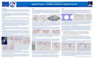
where ( ('2003/02/18 01:23:03' between startDateTime and endDateTime) or ('2003/02/18 03:03:57' between startDateTime and endDateTime) or ('2003/02/18 04:44:34' between startDateTime and endDateTime) or ('2003/02/18 06:05:21' between startDateTime and endDateTime) or ('2003/02/18 07:46:32' between startDateTime and endDateTime) or ('2003/02/18 12:47:46' between startDateTime and endDateTime) or ('2003/02/18 14:10:32' between startDateTime and endDateTime) or ('2003/02/18 15:51:02' between startDateTime and endDateTime) or ('2003/02/18 17:11:31' between startDateTime and endDateTime) or ('2003/02/18 18:52:07' between startDateTime and endDateTime) ) where startDateTime >= '1980/01/01 00:00:00' and endDateTime <= '2001/01/01 00:00:00' and ( (ascendingCrossing between -80.24 and -64.32) or (ascendingCrossing between 88.67 and 106.93) ) For the sea ice product (top, left) the polar stereographic projection was chosen because that’s what users are used to, and this specific region was chosen because there is no sea ice outside this region. But a lat/lon bounding box is a bad fit to the data coverage area as shown on a flat Earth (top, center) and the data’s native projection (top right). A spherical quadrilateral using only the corner points of the data (bottom, left) is a much better fit, but still has room for improvement. Because the coverage is at the data set level the consequences of being wrong are fairly severe. If a user happens to pick an area of interest that intersects the defined coverage area, but is outside the actual coverage area, every single granule in this dataset will be returned and all of it will be useless. The end result will be a greatly inconvenienced, and probably upset, user. Adding more points to the polygon slows performance but the area comparison is done only once for the entire data set, so performance isn’t much of an issue. Even if the comparison takes a whole hundredth of a second, that’s only one hundredth of a second. In this case it’s better to be accurate than fast and a spherical 20-gon (bottom, right) is much more accurate. Indeed, to really lock it down you might consider using every edge point, which in this case would be a spherical 1504-gon. National Snow and Ice Data Center Spatial Types: Looking Ahead to Spatial Search Ross Swick (swick@nsidc.org) http://geospatialmethods.org/search Introduction: Tiles: Orbits: Historically Relational Database Management Systems (RDBMSs) have not handled spatial information well. A lat/lon bounding box on a flat Earth was the best they could do, and good enough for most commercial needs. The Earth Science community has a different set of needs but, not being a major customer, had to make do with the flat Earth paradigm. That has changed in the last five years or so. These days most RDBMSs can handle a variety of spatial types on a spherical Earth, either natively or via a spatial extension, in fairly efficient ways. The Earth Science community now has an opportunity to improve the accuracy of the system by rethinking how spatial coverage is defined for different data types. And in order to take advantage of these new capabilities we need to make sure the required metadata are available. Tiled data is a special form of regional grid. A "tile" is a piece of a grid. It sometimes happens that the data are of such high resolution that the gridded product is much too large to include the entire grid in a single file. When that is the case the gridded product may be chopped into sub-grids typically by applying a much coarser lattice to the grid. For example the MODIS 500 meter resolution Northern and Southern Hemisphere Azimuthal product is chopped into (18x18 = 324) tiles, and the global Sinusoidal product is chopped into (18x36 = 648) tiles, just to keep the file sizes reasonable. Swath data are by far the most difficult data to work with when doing spatial search. As the satellite circles the rotating Earth a single orbit will cross all lines of longitude and most lines of latitudes. If the swath width of the sensor is wide enough the data will cover all longitudes and all latitudes, but only a small portion of the Earth's surface. The "unusual shape" of swath data (below, left) is often cited as the reason it is so difficult to work with. But the shape of a swath is only unusual if you look at it projected on a flat Earth (below, center). On spherical Earth (below, right) the shape of the swath is quite ordinary and much easier to work with. Points: Point data are data from a single point, generally in-situ measurements such as weather station data and ice cores. Point data are exactly the kind of data most RDBMSs are designed to handle and offers no challenges for spatial search. Often, however, point data are aggregated. If the aggregate is sparsely populated, as with weather station data in Northern Russia where the stations may be hundreds or even thousands of kilometers apart, most RDBMSs have a “multi-point” data type that may prove more useful than simply defining the entire area of coverage. For denser aggregates, preserving the pointiness of the data may be overkill. For example if multiple shallow cores are drilled during a field experiment it may be reasonable to define the coverage as the small area containing all the cores. Species sightings are another example where defining the coverage as an area may be reasonable. In those cases the spatial coverage is at the data set level and more appropriately handled at that level, as with gridded data. Indeed, if the points are dense enough that interpolating between them is a reasonable thing to do, the resulting product just is a gridded data set. Many methods for running a spatial search on swath data exist and each method requires defining the coverage of the swath using different parameters, so the two are intimately linked. This makes it important to decide what search method you are going to use prior to data production - so the data coverage can be appropriately described in the metadata that are ingested into the database. Two methods that don't work well, lat/lon bounding boxes and spherical polygons, are discussed above and we won't repeat that discussion here. Three other popular methods are: Predict orbit search, Nominal Orbit Spatial Extent (NOSE), and Backtrack orbit search. Predict orbit search methods rely on using an orbit model to predict when the satellite will be over the area of interest and consequently turn the spatial search into a temporal search. Predict methods are fast and accurate but are not well suited to long time series searches, which is something climate change research generally entails. Turning the spatial search into a temporal search means the temporal clause of the search has to be quite specific, and for long time series this clause can become quite large. For example polar orbiting satellites pass over or near Thule, Greenland 9 or 10 times per day, so a search for just a year’s worth of data over Thule would result in about 3600 specific times to search on. Even the temporal clause for a single day (top) is quite lengthy compared to the backtrack spatial clause (bottom) that works for any temporal range. So even though tiled data is a kind of gridded data it is not the case that every granule in the data set has the same spatial coverage. Still there is some regularity, every granule with the same tile coordinates does have the same spatial coverage, so there is no point doing a spatial search on each and every granule. The best way to do spatial search on tiled data is to run a spatial search on the tiles, then search the inventory by tile coordinates. This is best accomplished via a look-up table. In the example it would be a look-up table with less than 648 rows since some tiles are off the map and some products are land only or ocean only. Using a lookup table scheme, the spatial part of the search gets run on the tile set and a secondary search looks for granules with matching tile coordinates. Because the expensive spatial part of the search is limited to a few hundred tiles, instead of thousands of granules, the spatial coverage of the tiles can be defined more accurately without significantly degrading performance. Grids: Gridded data are data that have been processed into a predefined grid where a "grid" is defined as a lattice of a set resolution overlaid onto a projection. So a typical grid might be "Northern Hemisphere Azimuthal 25 km" indicating that a nominal 25 km resolution lattice has been overlaid on an azimuthal projection of the Northern Hemisphere. For many gridded data sets a lat/lon bounding box is sufficient and that method is still more efficient than spherical methods so it should be used when appropriate. Regional grids, however, are often not a good fit to a lat/lon bounding box as the choice of projection and/or subset of the grid often has more to do with the data, the region, or the user’s needs. Interpolated point data, for example, are often gridded to whatever projection best represents the region the points are in. And specific data products, such as the sea ice product pictured below, may cater to the needs of the user community. The key point for gridded data is that all granules in the data set are in the same grid, and consequently have the same coverage. So there is no need to do spatial search at the granule level. If the area of interest overlaps the grid then every granule overlaps the area of interest. Conversely if the area of interest does not overlap the grid there's no point doing a granule level search at all, since none of the granules overlap the area of interest. Tile 05v08h (left) from the sinusoidal grid is not a good fit to either a lat/lon bounding box (center) or a spherical quadrilateral (right) so a spherical polygon of more than four points is probably warranted. As with regional grids accuracy is more important than speed, but there are a few hundred tiles to search on so performance is more of an issue and one may want to limit the number of points in the polygon somewhat. The NOSE scheme relies on creating its own custom coordinate system for each data set. NOSE creates a set of nominal orbits, called “tracks”, for each sensor by creating a set of spherical polygons, called “blocks”, to define the coverage of the track. In practice there are usually 36 blocks per track, and to achieve a modest 1 degree accuracy there must be 360 tracks. The spatial coverage of each block is put in a lookup table which is used to determine what (track, block) coordinates cover the area of interest so a second search can search the inventory for granules that include those coordinates. The primary problem with NOSE is it is expensive. A new set of NOSE parameters must be developed for each sensor and preloaded into a lookup table, which ends up being quite large. To achieve a modest 1 degree accuracy the lookup table must have (36x360 = 12960) rows. A single track with 5 blocks outlined is pictured below Scenes: A "scene" is a small partial swath. Most environmental satellites have about a 100 minute period and often the data are divided into 5-minute scenes covering approximately 1/20th of an orbit or 18 degrees. Larger scenes are obviously possible and the difference between a scene and a partial swath is highly subjective. For example AVHRR LAC scenes (below, left) are captured by ground stations as the satellite passes overhead, and consequently are horizon-to-horizon (15 minutes, or about 54 degrees). For this scene a lat/lon bounding box is an incredibly poor fit (above, center) but a spherical rectangle (above, right) is a fairly good fit. Indeed defining the coverage of a scene as a spherical rectangle using only the corner points of the scene (above, right) will always include the entire scene, and always be a more accurate representation of the coverage area than the lat/lon bounding box. If greater accuracy is desired the coverage can be better defined by a spherical polygon using additional points from the edges of the scene. But running spatial searches on spherical polygons is cpu intensive so performance can become poor. Most RDBMSs use a number of heuristics to improve performance but these heuristics become less effective as the size of the scene increases. As mentioned above the point at which it is better to start using swath search methods is highly subjective but it is generally when the "scene" is larger than a quarter or third of an orbit. Backtrack is both cheaper to implement and more accurate than the NOSE scheme. Instead of creating a custom coordinate system for each data set Backtrack relies on the natural coordinate system of the data. Instead of predefined tracks Backtrack indexes swaths by the equator crossing longitude and does not use lookup tables. Backtrack starts with the area of interest and answers the question "If the sensor saw this area where must the satellite have crossed the equator?“ To do that Backtrack runs a simplified orbit model backwards from the area of interest to the equator crossing. In essence Backtrack defines the coverage of the orbit by defining the orbit (above, right), but to do that it does require that the crossing longitude be in the granule metadata. For more information see: http://geospatialmethods.org/search