Download
1 / 18
180 likes | 296 Views
Sensitivities of neutrino mixing parameters with atmospheric neutrinos at ICAL. Abhijit Samanta Harish-Chandra Research Institute Allahabad Based on arXiv 0812.4639 & 0812.4640(published in PRD). Content.

E N D
Sensitivities of neutrino mixing parameters with atmospheric neutrinos at ICAL Abhijit Samanta Harish-Chandra Research Institute Allahabad Based on arXiv 0812.4639 & 0812.4640(published in PRD)
Content Atmospheric neutrinos Oscillation of atmospheric neutrinos ICAL detector Oscillation analysis Migration from neutrino to muon Binning of the events Chi-square Systematic uncertainties Marginalization Sensitivities to 13, 23 |m232 | and octant of 23
Atmospheric neutrino flux & cross section Flux increases as we go to lower and lower E Deep inelastic event dominates at E 3 GeV for and E 7.5 GeV for Quasi-elastic cross section higher for than
Oscillation of atmospheric neutrinos In vacuum,
In matter, When MSW resonance occurs becomes large, also becomes large. ,
INO-ICAL Detector Mass: 50 kTon Size : 48 m (x) 16m (y) 12 m (z) 140 layers of 6 cm thick iron with 2.5 cm gap for active elements Magnetic field ~ 1 Tesla along y-direction There will be an option to change the active part of the detector .
Binning of the data • P is a function of (L/E) • 2. For a fixed E, the distance between two peaks in L increases with decrease of L • 3. For a fixed L, the distance between two peaks in E increases with increase of E • 4. Detector has finite E and L resolution. • 5. Oscillation effect can be seen well where the resolution width is smaller than • the distance between two peaks from oscillation. • It suggests binning in the grids of log E - log L.
Chi-square 4.8 GeV Total no. of bins ~ 1000. We have ensured no. of events ≥ 2 in each bin
Systematic uncertainties Uncertainty of
Deviation from bi-maximal mixing Octant discrimination Limits on 13
Comparison of different types of binning Log E- log L Log E -cosz Log (L/E)