Download
1 / 31
420 likes | 942 Views
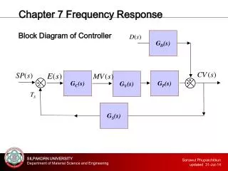
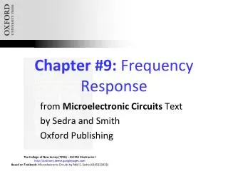
Chapter 9 Frequency Response and Transfer Function. § 9.1 Dynamic Signal in Frequency Domain § 9.2 Transfer Function and Frequency Response § 9.3 Representations of Frequency Transfer Function § 9.4 Frequency Domain Specifications of System Performance.

E N D
Chapter 9 Frequency Response and Transfer Function § 9.1 Dynamic Signal in Frequency Domain § 9.2 Transfer Function and Frequency Response § 9.3 Representations of Frequency Transfer Function § 9.4 Frequency Domain Specifications of System Performance
§9.1 Dynamic Signal in Frequency Domain (1) Laplace transform for one-sided function x(t) • Laplace Transform and Fourier Transform: Fourier transform for one-sided function x(t) Extension to two-sided Fourier Transform Laplace Transform is a one-sided generalized Fourier Transform with weighted convergent factor For one-sided function x(t), the Laplace transform is X(s). Then the Fourier Transform of x(t) is
§9.1 Dynamic Signal in Frequency Domain (2) (1) Periodic Signal --- Fourier Series Representation • Signal Decomposition and Representation: AC-components DC-component Periodic signal is represented as a combination of discrete sinusoidal signals. (2) Nonperiodic Signal --- Fourier Integral Representation Nonperiodic signal includes continuous frequency components with amplitude as spectral density.
§9.1 Dynamic Signal in Frequency Domain (3) • Classification of Dynamic Signal : Deterministic dynamic signal can be considered as a combination of different sinusoidal signals in discrete and/or continuous frequency spectrum.
§9.1 Dynamic Signal in Frequency Domain (4) • Frequency-Domain Representation :
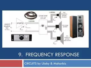
§9.1 Dynamic Signal in Frequency Domain (5) • Dynamic Signal and Measurement : Modern Spectrum Analyzer utilizes FFT (Fast Fourier Transform) algorithm for Real-time Fourier Transform.
§9.2 Transfer Function and Frequency Response (1) • Steady-state Sinusoidal Response :
§9.2 Transfer Function and Frequency Response (2) • Frequency Transfer Function (Frequency Response Function, FRF): Def: Ex: S.S. sinusoidal response and transmission of a mechanical system
§9.2 Transfer Function and Frequency Response (4) • Frequency Transfer Function and Pole-Zero Diagram :
§9.2 Transfer Function and Frequency Response (6) Rectangular Plot Polar Plot
§9.3 Representation of Frequency Transfer Function (1) • Definitions : Bode Plot – The plots of magnitude versus w in log-log rectangular coordinate and phase versus win semi-log rectangular coordinates, especially through corner plot or asymptotic plot. Power ratio Nyquist Plot – The plots of vectors in polar plot as is varied from zero to infinity.
§9.3 Representations of Frequency Transfer Function (2) • Formulation of Bode Plot G(jw) : Magnitude in dB: Phase: • Bode’s Gain-Phase Theorem: • For any stable minimum-phase system, the phase of is uniquely • related to the magnitude of . • The slope of the versus on a log-log scale is weighted most • heavily for the phase shift of a desired frequency. • (2) The log-log scale versus in one portion of the frequency • spectrum and the phase in the remainder of the spectrum • may be chosen independently.
§9.3 Representations of Frequency Transfer Function (3) Features of Bode’s Plot • can be constructed by the addition and subtraction of fundamental • building blocks in magnitude and phase, respectively. • Five fundamental building blocks: • (1) Constant gain • (2) Poles (zeros) at the origin • (3) Poles (zeros) on the real axis • (4) Complex poles (zeros) • (5) Pure time delay (lead) • 2. Same types of poles and zeros are mutual mirror images w.r.t. real axis.
§9.3 Representations of Frequency Transfer Function (4) • Bode Plot of Fundamental Building Blocks : • Constant Gain, G(s)=Kb • 2. Pure Integrator, Output amplitude is reduced as input frequency is increased.
§9.3 Representations of Frequency Transfer Function (5) 3. First order pole,
§9.3 Representations of Frequency Transfer Function (6) 4. Complex Poles
§9.3 Representations of Frequency Transfer Function (7) 5. Pure Time Delay
§9.3 Representations of Frequency Transfer Function (8) Ex: Magnitude: (1) 1stslope: -20 dB/decade (2) 2ndslope: 0 dB/decade (3) 3rdslope: -20 dB/decade (4) 4thslope: -40 dB/decade • Phase: • Starting from -90∘ • From APi to APf : increase 90∘ • From BPi to BPf : decrease 90∘ • From CPi to CPf : decrease 90∘ • Corner Phase: • P1: -45∘ • P2: -90∘ • P3: -135∘
§9.3 Representations of Frequency Transfer Function (9) • Non-minimum Phase G(jw) : A non-minimum phase all pass network G(s) pole-zero diagram Symmetric lattice network
§9.3 Representations of Frequency Transfer Function (10) • Phase Lead and Phase Lag Compensator : Phase Lead: Phase Lag: Lead and Lag Compensators are mutual mirror images w.r.t. real axis.
§9.3 Representations of Frequency Transfer Function (11) • General Shape of Nyquist Plot : Asymptotes: Low frequency High frequency
§9.3 Representations of Frequency Transfer Function (12) • Nyquist Plot of Fundamental Building Blocks : 1. Constant Gain, G(s)=Kb 4. Complex Poles, 2. Pure Integrator, 5. Pure Time Delay, 3. First-order Pole,
§9.3 Representations of Frequency Transfer Function (13) Ex: Polar plot of Ex: Polar plot of
§9.4 Frequency Domain Specifications of System Performance (1) • Frequency Response Test : Obtain the steady-state frequency response of a system to a sinusoidal input signal. Phase measurement by Lissajou Plot For nonlinear system, the output response is not in the same sinusoidal waveform and frequency as those of input signal.
§9.4 Frequency Domain Specifications of System Performance (2) • System Identification :
§9.4 Frequency Domain Specifications of System Performance (3) • Frequency-Domain Specifications :
§9.4 Frequency Domain Specifications of System Performance (4) For 1st-order pure dynamics For 2nd-order pure dynamics
§9.4 Frequency Domain Specifications of System Performance (5) Ex: Identify the structure modal parameters of the experimental FRF given by
§9.4 Frequency Domain Specifications of System Performance (6)