Download
1 / 28
350 likes | 629 Views
Supplier Relationship. 2002 년 11 월 29 일 금 김해중 MAI LAB. Contents. Relationship performance dimensions of buyer-supplier exchanges Production Quotas as Bounds on Interplant JIT Contracts. Relationship performance dimensions of buyer-supplier exchanges. Tom O’Toole*, Bill Donaldson**

E N D
Supplier Relationship 2002년 11월 29일 금 김해중 MAI LAB
Contents • Relationship performance dimensions of buyer-supplier exchanges • Production Quotas as Bounds on Interplant JIT Contracts
Relationship performance dimensions of buyer-supplier exchanges Tom O’Toole*, Bill Donaldson** *School of Accountancy and Business Studies, Waterford Institute of Technology, Waterford, Ireland **Graduate School of Business, University of Strathclyde, UK European Journal of Purchasing & Supply Management 8 (2002) 197~207
introduction • Relationship • 1970s in Europe. IMP(Industrial Marketing and Purchasing) group • Partnership management - Ellram, 1995 • Outsourcing strategic alliance - Mullin, 1996 • Supply chain co-operation and collaboration • Strategic role, potential relationship Supplier Buyer Objective A definition of buyer-supplier relationship performance Relational performance measures
B2B relationship performance • 3 Major problems • Lack of relationship performance from models • IMP group’s dyadic interaction(1982) • Dwyer et al: relationship development(1987) • Morgan and Hunt’s: commitment-trust model(1994) • Mohr and Spekman: model of partnership model(1994) • Anderson and Narus: distributor-manufacturing firm working partnership(1990) • Narrow definition of performance • Transaction cost • Cost savings for one party • Cost of potential relational abuses and the monitoring of a partnership • Theoretical borrowing • Financial perspective solely
The Study • Qualitative findings-explore dimensions • Interviews – 7 firms • 2 small, 2 medium, 3 large firms • 3 suppliers, 4 buyers • Financial/non-financial dimensions • Quantitative findings • Mail survey of 500 UK industrial buyers in manufacturing • 62% procurement managers, 19% managing director, 13% manufacturing manager, 6% others • 5-point scale, 21 items measuring performance • Response rate 47%, 200.
Non-financial performance statements • 다른 공급사와 비교해서 얻는 전반적인 이득은? • 납기 시간은? • 품질은? • 문제에 대한 반응 속도는? • 관계가 행복한가? (We are happy with this relationship) • 관계가 안정적인가? • 서로 합작 프로젝트를 수행하는가? • 제품 설계 시 협업을 하는가? • Financial performance statements • 다른 공급사로의 전환이 어려운가? switching cost • 관계가 서로 의존적일수록 더 이득인가? • 과도한 의존에 대해 대처가 쉬운가? • 정보와 지식을 공유해야만 하는가? • 비용절감은? • 지불하는 가격이 낮은가? • ROI는 높은가? • 장기 수익률은? • 비용 공유는? • 구매 물량은? • 운영비용은?
Findings and Discussion • correlations
Factor 1 • Speed of response • Product quality • Benefits comparison • Lead time Operational relationship effectiveness from buyer’s perspective Factor 2 • Satisfaction • Stability • Value diff. to quantify • Flexibility • Joint value projects Long-term interaction Strategic Factor 3 Close relationship • Involvement in design
Factor 1 • Switching • Interdependence • Cost sharing Measures of dependency Factor 2 • Confidence abuse • Share information Trust Factor 3 • Prices • ROI • Profitability • Bought volume • Cost of running Traditional economic measures
Conclusion • Financial / non-financial dimensions • Broadened conceptualization • Single actor perspectiveMutual Relationship
Production Quotas as Bounds on Interplant JIT Contracts Izak Deunyas*, Wallace J. Hopp**, Yehuda Bassok** *Department of Industrial and Operations Engineering, University of Michigan, Michigan **Department of Industrial Engineering and Management Sciences, Northwestern University, Illinois Management Science/ Vol.43, No.10 (1997)
Introduction(1/2) Clutch manufacturing plants • External supplier to US and Japanese car manufacturers • Demand is driven by production in downstream plant, stochastic Pull Production System Low Inventory High Responsive
Introduction(2/2) • 3 month ago: 1,404 units 2 month ago: 1,296 units a month ago: 9,396 units Actually 4,752 units Demand Uncertainty Ignore!! Visibility to future demand? No Objectives • Structure for the negotiated bounds on the JIT contracts • Optimal quota • Demand + Production variance cost + quota levels • Quota proposal for supplier
Literature Review • Card count-setting • Production quotas-setting • Optimal overtime policies • Uncertain capacity and demand • Single period • Optimal (s,c,S) policy Uncertain Demand Uncertain Production Safety Capacity Multi-period
OT decision is made RT OT RT OT Tn+1 Tn Un Dn is revealed Dn+1 is revealed Q D Q* Y t Model • Assumptions • Periodic production quota=target inventory level • Regular time + Safety capacity • Demand is uncertain • D>Q: Sales loss, D<Q:Holding cost
Notation • P : 제품 가격 • CR: 정규시간 동안의 비용 • C: overtime의 제품당 비용 • K: 잔업을 위한 setup비용 • Sn: 기초재고 n • Rn: 잔업 전의 재고 n • Dn: 수요 n. continuous density function fD, FD • Yn: 정규시간 동안의 생산용량 n fp, Fp • Q: 수익을 최대화하는 quota
RT OT Tn+1 Tn Un Tn+1 Overtime Un Production Q Rn Tn Inventory Sn Inventory level 기말재고 + Sn+1= (Q – Dn) 정규작업시간 후의 재고 Rn = min(Sn+Yn, Q) 기초재고 + Sn= (Q – Dn-1)
Profit maximization Profit n = Revenue - Regular cost - Overtime cost – Holding cost = p*min(Q, Dn) – CR*(Q-Sn) – K*Pr{Sn+Yn<Q} – C*(Q-Rn)–h*(Q-Dn-1)+ 판매수량 정규작업량 잔업 확률 잔업량 재고량 Long-term average profit per period Max G(Q) = (p-CR)E[min(Q, D)] – K*Pr{(Q-D)+ +Y<Q} - C*(Q - min[(Q - D)+ + Y , Q]) -hE(Q-D)+ Cost minimization Min W(Q) = p1E(D-Q)+ + hE(Q-D)+ + K*Pr{(Q-D)+ +Y<Q} + C*[Q - min[(Q - D)+ + Y , Q]) p1=(p-CR) Min W(Q)= - g(Q)+(p-CR)ED Marginal profit
First-order condition dW(Q)/dQ= 0 Second-order condition d2W(Q)/dQ2= 0 >0 Globally optimal Q* • Production • Demand f’p(x)>0 D=D+DX Unimodal Normal D 0 LP MP
Theorem 1 Q* is nonincreasing in K, h, c,non-decreasing in p 잔업/ 재고비용증가 Q 감소,가격상승Q 증가 Higher Price Supplier Customer Customer Supplier Q1 Q* Q1 Q* Q1=Q* Q1>Q*
Theorem 2 • Q*< D : K, h are is high enough D increases higher holding cost Q* decrease • Q*> D : marginal profit p1 is high enough D increasesneed more inventory as hedge Increase in D increase in the Q* Increase in Y increase in the Q* when K=0 Theorem 3 D=D+DX If Q*< D, Q* is non-increasing in D If Q*> D, Q* is non-decreasing in D
Alternative • The quota level desired by a customer How much additional capacity is required • m products on different, in compatible lines Theorem 4 Cv=D/D Q* is non-decreasing in D for a fixed Cv
Numerical example • Weekly demand from a manufacturer • D=D+DX= 100 + 20X • Y = P+PY= 125 + 10y • P1=1,k=75, c=0.4, h=0.05 • Q*=109.3 68% on time delivery P=130 ¼ D P=6 • Q*=106.4 fewer Q* theorem 3 • 90% on time delivery • Q*=115.3 • 94% on time delivery
Conclusion • Most of problems • Demand uncertainty >>production capacity uncertainty • Cost of demand uncertainty • Decreasing uncertainty can lead to benefits to both