Download
1 / 11
110 likes | 237 Views
GRAPH_1. ear. 12.0. y. , Gallons per. BUDGET CONSTRAINT AND INDIFFERENCE CURVE. Wine, (W). Price-consumption curve. e. 3. 5.2. e. 2. 4.3. 3. I. e. 1. 2.8. 2. I. 1. I. 1. L. (. p. = $12). 2. 3. L. (. p. = $6). L. (. p. = $4). b. b. b. 0. 26.7. 44.5.

E N D
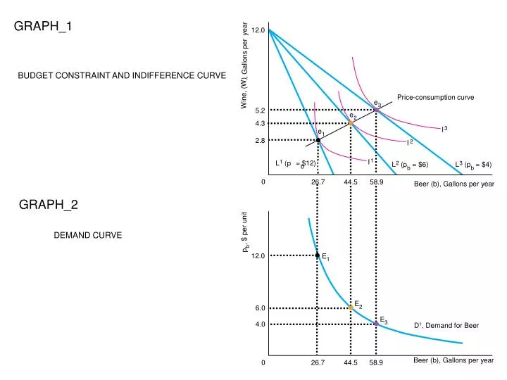
GRAPH_1 ear 12.0 y , Gallons per BUDGET CONSTRAINT AND INDIFFERENCE CURVE Wine, (W) Price-consumption curve e 3 5.2 e 2 4.3 3 I e 1 2.8 2 I 1 I 1 L ( p = $12) 2 3 L ( p = $6) L ( p = $4) b b b 0 26.7 44.5 58.9 Beer (b), Gallons per year GRAPH_2 , $ per unit DEMAND CURVE b p 12.0 E 1 E 2 6.0 E 3 4.0 D1, Demand for Beer Beer (b), Gallons per year 0 26.7 44.5 58.9
ear L3 y GRAPH_3 , Gallons per 2 L e BUDGET CONSTRAINT AND INDIFFERENCE CURVES Win 1 L Income-consumption curve e 3 7.1 e 4.8 2 I3 e 2.8 2 I 1 1 I 0 26.7 38.2 49.1 Bee r , Gallons per y ear , $ per unit GRAPH_4 r E E E 1 2 3 12 ice of bee DEMAND CURVE r P D3 2 D 1 D 0 26.7 38.2 49.1 Bee r , Gallons per y ear GRAPH_5 , Budget Engel curve for beer Y ENGEL CURVE * Y = $837 E 3 3 Y = $628 * E 2 2 Y = $419 * E 1 1 0 26.7 38.2 49.1 Bee r , Gallons per y ear
F ood in f e r io r , housing no r mal 1 IC C 2 L F ood no r mal, housing no r mal 2 IC C F ood no r mal, 3 IC C housing in f e r ior GRAPH_6 ear y eet per f a Housing, Square b 1 L e c I F ood, P ounds per y ear
3 L Y 3 Income-consumption cu r v e 2 L Y 2 e 3 3 I e 2 2 I , Income E3 Y Y E 2 2 Engel cu r v e Y 1 E 1 Ham b urger per y ear GRAPH_7A ear y All other goods per BUDGET CONSTRAINT AND INDIFFERENCE CURVES 1 L Y 1 e 1 1 I Ham b urger per y ear GRAPH_7B Y3 ENGEL CURVE
NORMAL GOOD CASE GRAPH_8 ear y L* , Units per s VD D vie o M D, 15 L1 L2 e* e1 e2 I1 I2 6 9 12 20 C , Music CDs Units per y ear Income effect = -3 Substitution effect = -3 Total effect = -6 = Substitution Effect + Income Effect = -3 + (-3)
2 L e 2 2 I e 1 1 I GIFFEN GOOD CASE I GRAPH_9A ear y ets per ck 1 L Ti etball, k Bas Total effect M o vie s , Ti ck ets per y ear
2 L e 2 2 I L * e 1 e * 1 I Substitution ef f ect Income ef f ect GIFFEN GOOD CASE II GRAPH_9B ear y ets per ck 1 L Ti etball, k Bas Total effect M o vie s , Ti ck ets per y ear
Time const r aint 2 I 2 L – w 2 1 I e 2 Y 2 1 L – w 1 e 1 Y 1 N = 12 N1 = 16 2 H = 12 H = 8 2 1 age per hour w W 2 , w w 1 N = 12 N1 = 16 2 H = 12 H = 8 2 1 (a) Indif f erence Cu r v es and Const r aints GRAPH_10 y a , Goods per d Budget constraint and Indifference curves Y 1 1 0 24 N , Leisure hours per day 24 0 H, Work hours per day (b) Demand Curve GRAPH_11 E 2 Demand for leisure E1 Demand for leisure N, Leisure hours per day 0 H, Work hours per day
L * e * Income and Substitution Effects of a Wage Change GRAPH_12 y Time const r aint a 2 I Since incomeeffect is positive, leisure is a normal good. 2 L , Goods per d 1 I Y e 2 1 L e 1 0 N * N N 24 N , Leisure hours per d a y 1 2 24 H * H H 0 H , W o r k hours per d a y 1 2 Substitution effect Total effect Income effect
3 L E 3 I 3 2 I E 2 e 3 2 L e 2 H H H H 2 3 2 3 Labor Supply Curve and Inferiority GRAPH_13 (a) Labor-Leisure Choice (b) Supply Cu r v e of Labor Supply curve of labor y a Time const r aint age per hour , Goods per d W , Y w 1 I E 1 1 L e 1 24 H 0 0 H 24 1 1 H , W o r k hours per d a y H , W o r k hours per d a y At low wages, an increase in the wage causes the worker to work more…. but at high wages, an increase in the wage causes the worker to work less….