Download
1 / 46
460 likes | 463 Views
This article explores the variability in the p53 signaling system and how mathematical models can help understand this phenomenon. It discusses the oscillatory dynamics and changing dynamics of the system, as well as the use of fluorescent microscopy in studying cellular components.

E N D
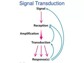
Example of Modeling Signal Transduction Systems Julie Dickerson
References and Readings • P53 Models and data: Oscillations and variability in the p53 system. Geva-Zatorsky N, Rosenfeld N, Itzkovitz S, Milo R, Sigal A, Dekel E, Yarnitzky T, Liron Y, Polak P, Lahav G, Alon U., Mol Syst Biol 2006;2:2006.0033. • Biomodels.net: database of models from publications • SBML.org: systems biology markup language definitions; links to tools and models
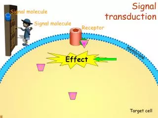
Biological Problem • In the p53 system, p53 transcriptionally activates mdm2. Mdm2, in turn, negatively regulates p53 by both inhibiting its activity as a transcription factor and by enhancing its degradation rate • The concentration of p53 increases in response to stress signals, such as DNA damage. The main mechanism for this increase is stabilization of p53 due to reduced interaction with Mdm2. • Following stress signals, p53 activates transcription of several hundred genes that are involved in growth arrest, apoptosis, senescence, and DNA repair. • Isogenic cells in the same environment behaved in highly variable ways following DNA-damaging gamma irradiation: some cells showed undamped oscillations for at least 3 days (more than 10 peaks). • Reference: Oscillations and variability in the p53 system. Geva-Zatorsky N, Rosenfeld N, Itzkovitz S, Milo R, Sigal A, Dekel E, Yarnitzky T, Liron Y, Polak P, Lahav G, Alon U., Mol Syst Biol 2006;2:2006.0033.
Modeling Problem • The amplitude of the oscillations was much more variable than the period. Sister cells continued to oscillate in a correlated way after cell division, but lost correlation after about 11 h on average. Other cells showed low-frequency fluctuations that did not resemble oscillations. • Why does this occur? Can models help us understand this? • Different families of mathematical models of the system point to the possible source of the variability in the oscillations: low-frequency noise in protein production rates, rather than noise in other parameters such as degradation rates. • Models available at: biomodels.net (numbers 154-159, curated models)
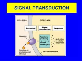
Transcriptional activation Negative regulation Inhibits transcription Enhances degradation
Also activates 100’s of genes: DNA repair Apoptosis Growth arrest Transcriptional activation Stress signals DNA Damage Negative regulation Inhibits transcription Enhances degradation
time time time Feedback loops • Oscillatory dynamics, changing dynamics monotone Damped Oscillations Sustained oscillation
P53 system • Studies with this system that used averages of cell responses showed damped oscillations following DNA damage. • Individual cell studies show a variation in responses in cells • Amplitudes changed, frequency did not change much
Fluorescent Microscopy • Fluorescence microscopy is one of the most used approaches in studying the location and movement of molecules and subcellular components in the cell. • Sample is itself the light source. • Based on the phenomenon that certain material emits energy detectable as visible light when irradiated with the light of a specific wavelength. • Samples can either be fluorescing in their natural form like chlorophyll and some minerals, or treated with fluorescing chemicals. • Usually, cellular components do not fluoresce themselves. Fluorescent markers are therefore introduced.
Fluorescent DyesFluorescent dyes are directly taken up by the cells. They are incorporated and concentrated in specific subcellular compartments. The living cells are then mounted on a microscope slide and examined. • ImmunofluorescenceImmunofluorescence involves the use of antibodies to which a fluorescent marker has been attached. Antibodies are molecules that recognize and bind selectively to specific target molecules in the cell. The fluorescent signal can be amplified by using an unlabelled primary antibody and detecting it with labelled secondary antibodies. • Tagging of ProteinsProtein molecules are tagged with a fluorescing marker. When a specific protein is modified in this way, the location of that protein can be studied. It is also possible to watch the movements of the proteins and its interactions with other cellular components inside the cell. http://nobelprize.org/educational_games/physics/microscopes/fluorescence/preparation.html
C. Elegans Nervous System The image shows the brain region of a living C. elegans animal. Different classes of neurons are labelled with different colors. Photo: H. Hutter, Max Planck Institut, Heidelberg Fluorescence triple-labeling of human cells. The DNA in two interphase cell nuclei (left and right) and in metaphase chromosomes from a third cell (middle) are shown in blue. Specific DNA sequences are labeled in red and green. Photo: Petra Björk, Stockholm University Fluorescence triple-labeling of human cells. Cytoplasmic fiber structures (microfilament) are shown in red. Components of the cell nuclei are shown in blue (nucleoli) and green (splicing factor). Photo: Petra Björk, Stockholm University Epithelium Cells Immunofluorescence staining of epithelium cell (Hep-2) mitochondria. (Zeiss)
Time Lapse microscopy of cells From supplementary data: Oscillations and variability in the p53 system. Geva-Zatorsky N, Rosenfeld N, Itzkovitz S, Milo R, Sigal A, Dekel E, Yarnitzky T, Liron Y, Polak P, Lahav G, Alon U., Mol Syst Biol 2006;2:2006.0033.
Prolonged oscillations in the nuclear levels of fluorescently tagged p53 and Mdm2 in individual MCF7, U280, cells following gamma irradiation. (A) Time-lapse fluorescence images of one cell over 29 h after 5 Gy of gamma irradiation. Nuclear p53-CFP and Mdm2-YFP are imaged in green and red, respectively. Time is indicated in hours. • (B) Normalized nuclear fluorescence levels of p53-CFP (green) and Mdm2-YFP (red) following gamma irradiation. Top left: the cell shown in panel A. Other panels: five cells from one field of view, after exposure to 2.5 Gy gamma irradiation. • Mol Syst Biol. 2006; 2: 2006.0033. • Published online 2006 June 13. doi: 10.1038/msb4100068.
Signal Analysis • Used Fourier analysis and spectrograms to estimate period of signals
Pitch (characteristic period) of Mdm2-YFP signals of cells at various gamma irradiation doses. (A) Histogram of the pitch values from movies of cells exposed to 0, 0.3, 5, and 10 Gy, and from all the movies together. For each movie, the total number of cells is indicated, and the number of oscillating (osc.) cells that had a detectable pitch. (B) Fraction of cells (out of the total number of cells) with a pitch value of 4–7 h, for different gamma doses. Black line is a guide to the eye. Mol Syst Biol. 2006; 2: 2006.0033. Published online 2006 June 13. doi: 10.1038/msb4100068.
Average amplitude, width, and time delay of oscillation peaks and their variance. (A–C) Average values of the first five p53-CFP (green triangles) and Mdm2-YFP (red squares) oscillation peaks in 146 cells exposed to 5 Gy of gamma irradiation, shown with their standard errors. (A) Average oscillation amplitude of each of the first five peaks (peak to trough). (B) Average width (full-width half-maximum). (C) Average time delay between the p53 peaks and the consecutive Mdm2 peak. Mol Syst Biol. 2006; 2: 2006.0033. Published online 2006 June 13. doi: 10.1038/msb4100068.
Modeling • Find simplest models that can explain these different behaviors • Negative feedback • Delay oscillators with delay in response to signals • Relaxation oscillators: negative feedback loop is supplemented with a positive loop on p53 • Checkpoint model, two negative feedback loops, direct and an effect on an upstream regulator of p53.
Describing Models • “Systems Biology Markup Language (SBML) is a computer-readable format for representing models of biochemical reaction networks in software. It's applicable to models of metabolism, cell-signaling, and many others.” (sbml.org)
Function definition • A named mathematical function that may be used throughout the rest of a model. • Unit definition • A named definition of a new unit of measurement, or a redefinition of an existing SBML unit. • Compartment Type • A type of location where reacting entities such as chemical substances may be located. • Species type • A type of entity that can participate in reactions. Typical examples of species types include ions such as Ca2+, molecules such as glucose or ATP, and more. • Compartment • A well-stirred container of a particular type and finite size where species may be located. A model may contain multiple compartments of the same compartment type. Every species in a model must be located in a compartment. • Species • A pool of entities of the same species type located in a specific compartment. • Parameter • A quantity with a symbolic name. In SBML, the term parameter is used in a generic sense to refer to named quantities regardless of whether they are constants or variables in a model.
Initial Assignment • A mathematical expression used to determine the initial conditions of a model. • Rule • A mathematical expression added to the set of equations constructed based on the reactions defined in a model. Rules can be used to define how a variable's value can be calculated from other variables, or used to define the rate of change of a variable. The set of rules in a model can be used with the reaction rate equations to determine the behavior of the model with respect to time. • Constraint • A means of detecting out-of-bounds conditions during a dynamical simulation and optionally issuing diagnostic messages. Constraints are defined by an arbitrary mathematical expression computing a true/false value from model variables, parameters and constants. • Reaction • A statement describing some transformation, transport or binding process that can change the amount of one or more species. For example, a reaction may describe how certain entities (reactants) are transformed into certain other entities (products). Reactions have associated kinetic rate expressions describing how quickly they take place. • Event • A statement describing an instantaneous, discontinuous change in a set of variables of any type (species quantity, compartment size or parameter value) when a triggering condition is satisfied.
Example • Identifier: EnzymaticReaction. • Compartment (with identifier cytosol) • four species (with identifiers ES, P, S, and E) • Reactions (veq and vcat). • Veq: • listOfReactants (E and S) and listOfProducts (ES). kinectic law • listOfParameters: kon and koff • Vcat: • listOfReactants (E S) and listOfProducts (E and P). kinectic law, not reversible. • listOfParameters: kcat
Model I • Delay Oscillator • Action of Mdm2 on p53 is linear, first-order kinetics x y0 y
Model III • Delay Oscillator • Action of Mdm2 has a delay term, production rate of Mdm2 depends on earlier value of p53
Model IV • Delay Oscillator • Action of Mdm2 on p53 is nonlinear, saturating Michaelis-Menten
Model II • Relaxation operator, positive feedback loop to upregulate p53
Model V • Relaxation operator, positive feedback loop to upregulate p53
S Model VI • Checkpoint • Mdm2 also affects a p53 precursor signaling protein, S, e.g., Phosphorylated ATM
Effect of cooperativity, n n increasing
Noise model • Periodic noise that varied in phase for protein production • Not white high frequency noise