Download
1 / 40
400 likes | 558 Views
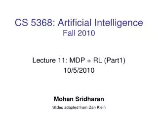
CS 5368: Artificial Intelligence Fall 2010. Lecture 11: MDP + RL (Part1) 10/5/2010. Mohan Sridharan Slides adapted from Dan Klein. Reinforcement Learning. Basic idea: Receive feedback in the form of rewards. Agent’s utility is defined by the reward function.

E N D
CS 5368: Artificial IntelligenceFall 2010 Lecture 11: MDP + RL (Part1) 10/5/2010 Mohan Sridharan Slides adapted from Dan Klein
Reinforcement Learning • Basic idea: • Receive feedback in the form of rewards. • Agent’s utility is defined by the reward function. • Must learn to act so as to maximize expected rewards.
Reinforcement Learning • Basic idea: • Receive feedback in the form of rewards. • Agent’s utility is defined by the reward function. • Must learn to act so as to maximize expected rewards. • Change the rewards, change the learned behavior! • Examples: • Playing a game, reward at the end for winning / losing • Vacuuming a house, reward for each piece of dirt picked up • Automated taxi, reward for each passenger delivered • First: Need to master MDPs.
Grid World • The agent lives in a grid. • Walls block the agent’s path. • The agent’s actions do not always go as planned: • 80% of the time, the action North takes the agent North (if there is no wall there). • 10% of the time, North takes the agent West; 10% East. • If there is a wall in the direction the agent would have been taken, the agent stays put. • Big rewards come at the end.
Markov Decision Processes • An MDP is defined by: • A set of states s S. • A set of actions a A. • A transition function T(s, a, s’): • Probability that a from s leads to s’. • P(s’ | s, a) – also called the model. • A reward function R(s, a, s’): • Sometimes just R(s) or R(s’). • A start state (or distribution). • Maybe a terminal state.. • MDPs are a family of non-deterministic search problems: • Reinforcement learning: MDPs where the T and R are unknown.
What is Markov about MDPs? • Andrey Markov (1856-1922) • “Markov” generally means that given the present state, the future and the past are independent. • For MDPs, “Markov” means:
Solving MDPs • In deterministic single-agent search problem, want an optimal plan, or sequence of actions, from start to goal. • In an MDP, we want an optimal policy *: S → A. • A policy gives an action for each state. • An optimal policy maximizes expected utility if followed. • Defines a reflex agent. Optimal policy when R(s, a, s’) = -0.03 for all non-terminals s.
Example Optimal Policies R(s) = -0.03 R(s) = -0.01 R(s) = -2.0 R(s) = -0.4
Example: High-Low • Three card types: 2, 3, 4. • Infinite deck, twice as many 2’s. • Start with 3 showing. • Say “high” or “low” after each card. • New card is flipped: • If you are right, you win the points shown on the new card. • If you are wrong, game ends. • Ties are no-ops. • Differences from expectimax: • #1: get rewards as you go. • #2: you might play forever! 3 4 2 2
High-Low • States: 2, 3, 4, done. Start: 3. • Actions: High, Low. • Model: T(s, a, s’): • P(s’=done | 4, High) = 3/4 • P(s’=2 | 4, High) = 0 • P(s’=3 | 4, High) = 0 • P(s’=4 | 4, High) = 1/4 • P(s’=done | 4, Low) = 0 • P(s’=2 | 4, Low) = 1/2 • P(s’=3 | 4, Low) = 1/4 • P(s’=4 | 4, Low) = 1/4 • … • Rewards: R(s, a, s’): • Number shown on s’ if s s’. • 0 otherwise. 4 Note: could choose actions with search. How?
High Low 3 3 , High , Low T = 0.25, R = 3 T = 0, R = 4 T = 0.25, R = 0 T = 0.5, R = 2 3 2 4 High Low High Low Low High Example: High-Low 3
MDP Search Trees • Each MDP state gives an expectimax-like search tree. s is a state s a (s, a) is a q-state s, a (s,a,s’) called a transition T(s,a,s’) = P(s’|s,a) R(s,a,s’) s,a,s’ s’
Utilities of Sequences • In order to formalize optimality of a policy, need to understand utilities of sequences of rewards. • Typically consider stationary preferences: • Theorem: only two ways to define stationary utilities • Additive utility: • Discounted utility: Assuming that reward depends only on state for these slides!
Infinite Utilities?! • Problem: infinite sequences with infinite rewards. • Solutions: • Finite horizon: • Terminate after a fixed T steps. • Gives non-stationary policy ( depends on time left). • Absorbing state(s): guarantee that for every policy, agent will eventually “die” (like “done” for High-Low). • Discounting: for 0 < < 1. • Smaller means smaller “horizon” – shorter term focus.
Discounting • Typically discount rewards by < 1 in each time step: • Sooner rewards have higher utility than later rewards. • Also helps the algorithms converge!
s a s, a s,a,s’ s’ Optimal Utilities • Fundamental operation: compute the optimal utilities of states s. • Define the utility of a state s: V*(s) = expected return starting in s and acting optimally. • Define the utility of a q-state (s,a): Q*(s,a) = expected return starting in s, taking action a and thereafter acting optimally. • Define the optimal policy: *(s) = optimal action from state s.
Optimal Policies and Utilities • Expected utility with executing starting in s: • Optimal policy: • One-step: choose action to maximize expected utility of next state:
s a s, a s,a,s’ s’ The Bellman Equations • Definition of “optimal utility” leads to a simple one-step look-ahead relationship amongst optimal utility values: Optimal rewards = maximize over first action and then follow optimal policy. • Formally:
The Bellman Equations • Iterative Bellman updates to arrives at optimal values and policies. • Formal definition of optimal functions: • Next: how to choose actions? how to compute the optimal policy?
Computing Actions • Which action should we chose from state s: • Given optimal values V? • Given optimal q-values Q? • Lesson: actions are easier to select from Q’s!
s a s, a s,a,s’ s’ Solving MDPs • We want to find the optimal policy* • Proposal 1: modified expectimax search, starting from each state s.
Recap: MDP Search Trees • Each MDP state gives an expectimax-like search tree. s is a state s a (s, a) is a q-state s, a (s,a,s’) called a transition T(s,a,s’) = P(s’|s,a) R(s,a,s’) s,a,s’ s’
Why Not Search Trees? • Why not solve with expectimax? • Problems: • This tree is usually infinite (why?). • Same states appear over and over (why?). • We search once per state (why?). • Idea: Value iteration • Compute optimal values for all states all at once using successive approximations. • Will be a bottom-up dynamic program similar in cost to memoization. • Do all planning offline, no replanning needed!
Value Estimates • Calculate estimates Vk*(s) • Not the optimal value of s. Considers only next k time steps. • Optimal value as k . • Why does this work? • With discounting, distant rewards become negligible. • If terminal states reachable from everywhere, fraction of episodes not ending becomes negligible. • Otherwise, can get infinite expected utility. Then this approach will not work.
Value Iteration • Idea: • Start with V0*(s) = 0, which we know is right (why?) • Given Vi*, calculate the values for all states for depth i+1: • This is called a value update or Bellman update. • Repeat until convergence. • Theorem: will converge to unique optimal values! • Basic idea: approximations get refined towards optimal values. • Policy may converge long before values do!
Example: =0.9, living reward=0, noise=0.2. Example: Bellman Updates Max happens for a=right, other actions not shown.
Example: Value Iteration V2 V3 • Information propagates outward from terminal states and eventually all states have correct value estimates.
0.705 Eventually: Correct Values V3 (when R=0, =0.9) V* (when R=-.04, =1) • This is the unique solution to the Bellman Equations! 0.52 0.78 0.812 0.868 0.918 0.43 0.660 0.762 0.655 0.611 0.388
Convergence of Value Iteration* • Define the max-norm: • Theorem: For any two approximations U and V: • I.e. any distinct approximations must get closer to each other, so, in particular, any approximation must get closer to the true U and value iteration converges to a unique, stable, optimal solution. • Theorem: • I.e. once the change in our approximation is small, it must also be close to correct.
Computing Actions • Which action should we chose from state s: • Given optimal values V? • Given optimal q-values Q? • Lesson: actions are easier to select from Q’s! • How do we compute policies based on Q-values?
Diversion: Utilities for a Fixed Policy • Another basic operation: compute the utility of a state s under a fix (general non-optimal) policy • Define the utility of a state s, under a fixed policy : V(s) = expected total discounted rewards (return) starting in s and following • Recursive relation (one-step look-ahead / Bellman equation): s (s) s, (s) s, (s),s’ s’
Policy Evaluation • How do we calculate the V’s for a fixed policy? • Idea 1: turn recursive equations into updates: • Idea 2: it is just a linear system, solve with Matlab (or whatever). • Both ideas are valid solutions.
Policy Iteration • Problem with value iteration: • Considering all actions in each iteration is slow: takes |A| times longer than policy evaluation. • But policy does not change each iteration, i.e., time is wasted • Alternative to value iteration: • Step 1: Policy evaluation: calculate utilities for a fixed policy (not optimal utilities!) until convergence (fast!). • Step 2: Policy improvement: update policy using one-step look-ahead with resulting converged (but not optimal!) utilities (slow but infrequent). • Repeat steps until policy converges. • This is policy iteration: • It is still optimal! Can converge faster under some conditions
Policy Iteration • Policy evaluation: with fixed current policy , find values with simplified Bellman updates: • Iterate until values converge. • Policy improvement: with fixed utilities, find the best action according to one-step look-ahead.
Comparison • In value iteration: • Every pass (or “backup”) updates both utilities (explicitly, based on current utilities) and policy (possibly implicitly, based on current policy). • In policy iteration: • Several passes to update utilities with frozen policy. • Occasional passes to update policies. • Hybrid approaches (asynchronous policy iteration): • Any sequences of partial updates to either policy entries or utilities will converge if every state is visited infinitely often.
Asynchronous Value Iteration* • In value iteration, update every state in each iteration. • Actually, any sequence of Bellman updates will converge if every state is visited infinitely often. • In fact, we can update the policy as seldom or often as we like, and we will still converge! • Idea: Update states whose value we expect to change: If is large, update predecessors of s.
Reinforcement Learning • Reinforcement learning: • Still have an MDP: • A set of states s S • A set of actions (per state) A • A model T(s, a, s’) • A reward function R(s, a, s’) • Still looking for a policy (s) • New twist: don’t know T or R. • I.e. don’t know which states are good or what the actions do. • Must actually try actions and states out to learn.
Example: Animal Learning • RL studied experimentally for more than 60 years in psychology. • Rewards: food, pain, hunger, drugs, etc. • Mechanisms and sophistication debated. • Example: foraging. • Bees learn near-optimal foraging plan in field of artificial flowers with controlled nectar supplies. • Bees have a direct neural connection from nectar intake measurement to motor planning area.
Example: Backgammon • Reward only for win / loss in terminal states, zero otherwise. • TD-Gammon learns a function approximation to V(s) using a neural network. • Combined with depth 3 search, one of the top 3 players in the world! • You could imagine training Pacman this way… but it’s tricky!
What next? • Types of problems in RL: • Model-based, Model-free. • Active, Passive. • Popular solution techniques: • Q-learning. • Temporal-difference (TD) methods.