Download
1 / 23
230 likes | 307 Views
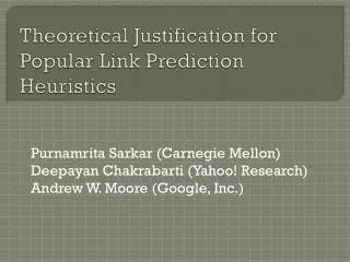
A Theoretical Justification of Link Prediction Heuristics. Deepayan Chakrabarti (deepay@cs.cmu.edu). Purnamrita Sarkar. Andrew Moore. Link Prediction. Which pair of nodes {i,j} should be connected?. Alice. Bob. Charlie. Goal: Recommend a movie. Link Prediction.

E N D
A Theoretical Justification of Link Prediction Heuristics DeepayanChakrabarti (deepay@cs.cmu.edu) PurnamritaSarkar Andrew Moore
Link Prediction • Which pair of nodes {i,j} shouldbe connected? Alice Bob Charlie Goal: Recommend a movie
Link Prediction • Which pair of nodes {i,j} shouldbe connected? Goal: Suggest friends
Link Prediction Heuristics • Predict link between nodes • Connected by the shortest path • With the most common neighbors (length 2 paths) • More weight to low-degree common nbrs (Adamic/Adar) Prolific common friends Less evidence Alice Less prolific Much more evidence 1000 followers Bob Charlie 3followers
Link Prediction Heuristics • Predict link between nodes • Connected by the shortest path • With the most common neighbors (length 2 paths) • More weight to low-degree common nbrs (Adamic/Adar) • With more short paths (e.g. length 3 paths ) • exponentially decaying weights to longer paths (Katz measure) • …
Previous Empirical Studies* Especially if the graph is sparse How do we justify these observations? Link prediction accuracy* Random Shortest Path Common Neighbors Adamic/Adar Ensemble of short paths *Liben-Nowell & Kleinberg, 2003; Brand, 2005; Sarkar & Moore, 2007
Link Prediction – Generative Model Unit volume universe Model: • Nodes are uniformly distributed points in a latent space • This space has a distance metric • Points close to each other are likely to be connected in the graph • Logistic distance function (Raftery+/2002)
Link Prediction – Generative Model α determines the steepness 1 ½ radius r Model: Nodes are uniformly distributed points in a latent space This space has a distance metric Points close to each other are likely to be connected in the graph Higher probability of linking • Link prediction ≈ find nearest neighbor who is not currently linked to the node. • Equivalent to inferring distances in the latent space
Previous Empirical Studies* Especially if the graph is sparse Link prediction accuracy* Random Shortest Path Common Neighbors Adamic/Adar Ensemble of short paths *Liben-Nowell & Kleinberg, 2003; Brand, 2005; Sarkar & Moore, 2007
Common Neighbors • Pr2(i,j) = Pr(common neighbor|dij) j i Product of two logistic probabilities, integrated over a volume determined by dij Asα∞Logistic Step function Much easier to analyze!
Common Neighbors Everyone has same radius r Unit volume universe j i η=Number of common neighbors V(r)=volume of radius r in D dims # common nbrs gives a bound on distance
Common Neighbors • OPT = node closest to i • MAX = node with max common neighbors with i • Theorem: w.h.p dOPT ≤ dMAX≤ dOPT + 2[ε/V(1)]1/D Link prediction by common neighbors is asymptotically optimal
Common Neighbors: Distinct Radii j k • Node k has radius rk . • ik if dik ≤ rk (Directed graph) • rk captures popularity of node k i rk i j m k j k i Type 2: i k j Type 1: i k j rj rk rk ri A(ri, rj,dij) A(rk , rk,dij)
Type 2 common neighbors • Example graph: • N1 nodes of radius r1 and N2 nodes of radius r2 • r1 << r2 k i j η2 ~ Bin[N2 , A(r2, r2, dij)] η1 ~ Bin[N1 , A(r1, r1, dij)] Pick d* to maximize Pr[η1 , η2 | dij] w(r1)E[η1|d*] + w(r2) E[η2|d*] = w(r1)η1 + w(r2) η2 Weighted common neighbors Inversely related to d*
Common Neighbors: Distinct Radii j k • Node k has radius rk . • ik if dik ≤ rk (Directed graph) • rk captures popularity of node k • “Weighted” common neighbors: • Predict (i,j) pairs with highest Σ w(r)η(r) i rk m # common neighbors of radius r Weight for nodes of radius r
Type 2 common neighbors j k i rk Adamic/Adar Presence of common neighbor is very informative Absence is very informative 1/r r is close to max radius Real world graphs generally fall in this range
Previous Empirical Studies* Especially if the graph is sparse Link prediction accuracy* Random Shortest Path Common Neighbors Adamic/Adar Ensemble of short paths *Liben-Nowell & Kleinberg, 2003; Brand, 2005; Sarkar & Moore, 2007
l hop Paths • Common neighbors = 2 hop paths • Analysis of longer paths: two components • Bounding E(ηl | dij).[ηl= # l hop paths] • Bounds Prl (i,j) by using triangle inequality on a series of common neighbor probabilities. • ηl≈E(ηl | dij) • Triangulation
l hop Paths • Common neighbors = 2 hop paths • Analysis of longer paths: two components • Bounding E(ηl | dij).[ηl= # l hop paths] • Bounds Prl (i,j) by using triangle inequality on a series of common neighbor probabilities. • ηl≈E(ηl | dij) • Bounded dependence of ηlon position of each node Can use McDiarmid’s inequality to bound|ηl-E(ηl|dij)|
ℓ-hop Paths • Common neighbors = 2 hop paths • For longer paths: • Bounds are weaker • For ℓ’ ≥ℓwe need ηℓ’ >> ηℓto obtain similar bounds • justifies the exponentially decaying weight given to longer paths by the Katz measure
Summary • Three key ingredients • Closer points are likelier to be linked. Small World Model- Watts, Strogatz, 1998, Kleinberg 2001 • Triangle inequality holds necessary to extend to ℓ-hop paths • Points are spread uniformly at random Otherwise properties will depend on location as well as distance
Summary In sparse graphs, paths of length 3 or more help in prediction. Differentiating between different degrees is important For large dense graphs, common neighbors are enough Link prediction accuracy* The number of paths matters, not the length Random Shortest Path Common Neighbors Adamic/Adar Ensemble of short paths *Liben-Nowell & Kleinberg, 2003; Brand, 2005; Sarkar & Moore, 2007
Sweep Estimators Number of common neighbors of a given radius r TR = Fraction of nodes with radius ≥ R which are common neighbors Qr = Fraction of nodes with radius ≤ r which are common neighbors Large Qr small dij Small TR large dij