Download
1 / 42
420 likes | 511 Views
Required Sample size for Bayesian network Structure learning. Samee Ullah Khan and Kwan Wai Bong Peter. Outline. Motivation Introduction Sample Complexity Sanjoy Dasgupta Russell Greiner Nir Friedman David Haussler Summary Conclusion. Motivation.

E N D
Required Sample size for Bayesian network Structure learning Samee Ullah Khan and Kwan Wai Bong Peter
Outline • Motivation • Introduction • Sample Complexity • Sanjoy Dasgupta • Russell Greiner • Nir Friedman • David Haussler • Summary • Conclusion
Motivation • John Works at a Pharmaceutical Company. • Optimal Sample Size of a Clinical Trial? • It’s a function of Both Statistical Significance of the Difference and the Magnitude of Apparent difference between Performances. • Purpose: A tool (measure) for Public and Commercial vendors to plan clinical trials. • Looking For: Gain acceptance from potential users. • Statistically Significance Evidence
Motivation: Solution • Optimize the difference between the performances of both treatments. • Let C= diff (expected cost of new treatment –expected cost of old treatment)
Motivation • C=0, m= users, is the difference in performance
Motivation • C>0
Motivation • C<0
Motivation: Conclusion • Actual improvement in performance is known • It may be extended to the uncertainty about the amount of improvement. • It is also possible to shift the functions 1` or 2`to right. • Where ` is standard deviation of the posterior distribution of unknown parameter .
Motivation: Model • Paired Observations (X1,Y1),(X2,Y2)…….. • Xi is new clinical outcome • Yi is old clinical outcome • Let Z be the objective function • Zi=Xi-Yi (i=1,2,3……….) • Assume that has normal density N(,2) • Formulating our previous knowledge about assume a prior density N(,2). • Under the assumptions is a sufficient statistics for the parameter .
Introduction • Efficient learning -- more accurate models with less data • Compare: P(A) and P(B) vs joint P(A,B) former requires less data! • Discover structural properties of the domain • Identifying independencies in the domain helps to • Order events that occur sequentially • Sensitivity analysis and inference • Predict effect of actions • Involves learning causal relationship among variables
Introduction • Why Struggle for Accurate Structure
Introduction • Adding an Arc • Increases the number of parameters to be fitted • Wrong assumptions about causality and domain structure
Introduction • Deleting an Arc • Cannot be compensated by accurate fitting of parameters • Also misses causality and domain structure
Introduction • Approaches to Learning Structure • Constraint based • Perform tests of conditional independence • Search for a network that is consistent with the observed dependencies and independencies • Score based • Define a score that evaluates how well the (in)dependencies in a structure match the observations • Search for a structure that maximizes the score
Introduction • Constraints versus Scores • Constraint based • Intuitive, follows closely the definition of BNs • Separates structure construction from the form of the independence tests • Sensitive to errors in individual tests • Score based • Statistically motivated • Can make compromises • Both • Consistent---with sufficient amounts of data and computation, they learn the correct structure
Dasgupta’s model • Haussler’s extension of the PAC framework • Situation: fixed network structure • Goal: To learn the conditional probability functions accurately
Dasgupta’s model • A learning algorithm A: • Given: • An approximation parameter > 0 • A confidence parameter 0 < < 1 • Variables drawn from a instance space X, x1, x2, …, xn • An oracle which generates randomly instances of X according to some unknown distribution P that we are going to learn • Some hypothesis class H
Dasgupta’s model • Output: hypothesis h H such that with probability > 1- where d(.,.) is a distance measure hopt is the concept h’ H that minimizes d(P, h’)
Dasgupta’s model: Distance measure • Most intuitive: L1 norm • Most popular: Kullback-Leibler divergence (relative entropy) • Minimizing dKL with respect to the empirically observed distribution is equivalent to solving the maximum likelihood problem
Dasgupta’s model: Distance measure • Disadvantage of dKL: unbounded • So, the measure adopted in this model is relative entropy by replacing log with ln.
Dasgupta’s model • The algorithm, given m samples drawn from some distribution P, finds the best fitting hypothesis by evaluating each h(,)H(,) by computing the empirical log loss E(-ln h(,)) and returning the hypothesis with the smallest value, where H(,)H, called an (,)-bounded approximation of H.
Dasgupta’s model • By using Hoeffding and Chernoff bounds, the number of samples needed is bounded by • Lower bound:
Rusell Greiner’s claim • Many learning algorithms that determine which Bayesian network is optimal usually based on some measures such as log-likelihood, MDL, BIC. These typical measures are independent of the queries that will be posed. • Learning algorithms should consider the distribution of queries as well as the underlying distribution of events, and seek the BN with the best performance over the query distribution rather than the one that appears closest to the underlying event distribution.
Russell Greiner’s model • Let V: set of the N variables SQ: set of all possible legal statistical queries sq(x; y): a distribution over SQ • Suppose we fixed a network B over V, and let B(x|y) be the real-value probability that B returns for this assignment. Given distribution sq(.,.) over SQ, the “score” of B is • err(B)=errsq,p(B) if sq, p are clear from context
Russell Greiner’s model • Observation: • Any Bayesian network B* that encodes the underlying distribution p(.), will in fact produce the optimal performance; i.e. err(B*) will be optimal • This means that if we have a learning algorithm that produces better approximations to p(.) as it sees more training examples, then in the limit the sq(.) distribution becomes irrelevant.
Russell Greiner’s model • Given a set of labeled statistical queries Q={<xi;yi;pi>}i, let be the empirical score of the Bayesian net.
Russell Greiner’s model • Compute err(B): • #P-hard to compute the estimate of err(B) from general statistical queries • If we know that all queries encountered sq(x;y), satisfy p(y) for some >0, then we only need complete event examples, with example queries to obtain an -close estimate, with probability at least 1-.
Nir Friedman’s model • Review • BN is composed of two parts. • DAG • Parameters encoding • Setup • Let B* be a BN that describe the target distributions from training samples. • Entropy Distance (Kullback-Leibler) • Learn from Random Variables, decrease with N.
Nir Friedman’s model: Learning • Criteria: • Error Threshold • Confidence Threshold • N(,) sample size • If the sample size is larger than N(,) then Pr(D(PLrn()||P)>)< where Lrn() represents the learning routine. • If N(,) is MINIMAL the it is called sample complexity.
Nir Friedman’s model:Notations • Vector Valued U={X1, X2,……Xn} • X,Y,Z Variables • x,y,z values • So B=<G,> • G is DAG • are number of parameters • xi|xi =P(xi|xi) • BN is minimal
Nir Friedman’s model:Learning • Given a training set wN={u1,……..un} of U find B that best matches D. • The loglikelihood of B: • Decomposing loglikelihood according to structure:
Nir Friedman’s model:Learning • So we can derive • Assume G has fixed structure, optimize • Argument is large networks not desirable
Nir Friedman’s model: PSM • Penalized weighting function: • MDL principle: • Total description length of data • AIC • BIC
Nir Friedman’s model: Sample Complexity • Sample complexity • Log-likelihood and penality term • Random noise • Entropy distance
Nir Friedman’s model: Sample Complexity • Idealized case
Nir Friedman’s model: Sample Complexity • Sub-sampling strategies in learning
Nir Friedman’s model: Summary • It can be shown on the sample complexity of BN using MDL • Bound is loose • To search for an optimal structure is NP-hard
David Haussler’s model • The model is based on prediction. The learner attempts to infer an unknown target concept f chosen from a concept class F of {0, 1} valued function. • For any given instance i, the learner predicts value of f(xi). • After the prediction, the learner is to the correct answer. It improves on the result.
David Haussler’s model • Criteria for sample bounds: • Probability of f(xm+1) over (x1, f(x1)), …,(xm,f(xm)) • Cumulative mistakes made over m trials • The model uses VC dimension
VC • General condition for uniform convergence: • Definition: • Shattered set. Let X be the instance space and C the concept class • SX, shattered by C • S’ S, c C which contains all S’ and none of S-S’ • SX, C(S) S
David Haussler’s model • Information Gain • At instance m, the learner has observed f(x1),…,f(xm) labels predict f(xm+1)