Download
1 / 16

E N D
Chapter 12 – Chi Square Tests • We have done tests on population means and population proportions. However, it is possible to test for population variances. Also, it is necessary to test if an observed frequency is different from an expected frequency and if a variable is independent of another variable. These three tests are covered in Chapter 12. • When performing these tests, we use a different type of distribution. This is known as chi-square (pronounced as kai-square) distribution.
A chi-square distribution • A chi-square distribution is shown in figure 12-1, on page 372. The shape of the curve depends on sample size. • Appendix F (pages 482-483) presents probabilities of chi-square distribution.
Tests for population variance • The test statistic for these tests is: 2 2 (n – 1) s X = ------------- 2 σ • The two hypotheses are: Ho: σ2= given value; H1: σ2 > given value < given value ≠ given value
Tests for pop. var. (Cont) • The decision rule is the same as before Example problem 12-1 page 310. 2 X = 11.25 • Critical x2 from appendix F for 9 Degrees of freedom & alpha ( α ) of 0.01 is 21.666. • Decision: Do not reject H0.
Interpretation: • The variance in breaking strength of the cable has remained the same (at most 40,000 pounds).
Problem 10, pg 312 Given: n = 6 s2 = 91.6 σ2=100 α = 0.1 H : σ2 = 100 H : σ2 < 100 o 1
Problem 10, cont. • Decision rule: Reject H0 if x2 < critical x2 (5, 1-0.1) X2 = [(6-1)91.6]/100 = 4.58 Critical x2 from appendix F is 1.61031 • Be careful of how to find critical x2 from appendix F
Decision: Do not reject H0 • Interpretation: The weight gain for the specific breed of sheep is equally uniform (That is the variance in weight gain is equal to 100).
Testing for goodness of fit • In some experiments, we are interested in knowing if observed frequencies are same as expected frequencies. For example, we toss a coin 100 times. We expect that we will get 50 heads and 50 tails. Now, suppose we observed 45 heads and 55 tails. Can we still say that the coin is balanced?
Testing for goodness of fit (Con’t) • These types of tests are called goodness of fit tests. The words expected and observed frequencies are important. • Two hypotheses are: H0: observed frequencies are the same as expected frequencies H1: Observed frequencies are not the same as expected frequencies
The test statistic is: 2 2 (O - E ) X = ∑--------------- E • Where Oj are observed frequencies Ej are expected frequencies • Decision Rules (Always of this form): 2 Reject H0 if X-Statistic is > Critical x2
The test statistic (con’t) • The degrees of freedom is number of rows minus 1. Refer to table 12-2 on page 314. The degrees of freedom is 6-1= 5. Example problem 12-4, page 315-316. • Refer to table 12-3 on page 315 • The hypotheses are:H0: voters today have the same education attainment as those 20 years agoH1: Voters today do not have the same educational attainment as those 20 years ago
The test statistic • X2-statistic = 19.25 • Critical x2 with 4 degrees of freedom and alpha of 0.05 is 9.48773. • Decision: reject H0 • Interpretation:Voters today do not have the same education attainment as those 20 years ago.
Exercises from book Problem 6 on page 316-317 • The 2 hypotheses are: H0: Saturday & Sunday each accounts for 25% and each of the 5 remaining days accounts for 10% of all fatal accidents H1: Sat & Sun do not each account…and each of the 5 remaining days do not account for 10% of all fatal accidents
Exercises • Use alpha = 0.025 • N= 7 so degree of freedom = 7-1 = 6 • Decision rule: Reject H0 if X2 > critical x2(6,0.025) X2 = 2.2 2 • Critical X = 14.4494 (from Appendix F)
Decision and interpretation • Decision: Do not reject H0 • Interpretation: Sat & Sun each accounts for 25% & each of the 5 weekdays accounts for 10% of all fatal accidents of the LA freeways