Download
1 / 21
270 likes | 614 Views
Chapter 3, Numerical Descriptive Measures. Data analysis is objective Should report the summary measures that best meet the assumptions about the data set Data interpretation is subjective Should be done in fair, neutral and clear manner. Summary Measures. Describing Data Numerically.

E N D
Chapter 3, Numerical Descriptive Measures • Data analysis is objective • Should report the summary measures that best meet the assumptions about the data set • Data interpretation is subjective • Should be done in fair, neutral and clear manner
Summary Measures Describing Data Numerically Central Tendency Variation Shape Arithmetic Mean Range Skewness Median Interquartile Range Mode Variance Geometric Mean Standard Deviation Coefficient of Variation Quartiles
Arithmetic Mean • The arithmetic mean (mean) is the most common measure of central tendency • Mean = sum of values divided by the number of values • Affected by extreme values (outliers) Sample size Observed values
Geometric Mean • Geometric mean • Used to measure the rate of change of a variable over time • Geometric mean rate of return • Measures the status of an investment over time • Where Ri is the rate of return in time period I
Median: Position and Value • In an ordered array, the median is the “middle” number (50% above, 50% below) • The location (position) of the median: • The value of median is NOT affected by extreme values
Mode • A measure of central tendency • Value that occurs most often • Not affected by extreme values • Used for either numerical or categorical data • There may may be no mode • There may be several modes
Quartiles • Quartiles split the ranked data into 4 segments with an equal number of values per segment • Find a quartile by determining the value in the appropriate position in the ranked data, where First quartile position: Q1 = (n+1)/4 Second quartile position: Q2 =2 (n+1)/4 (the median position) Third quartile position: Q3 = 3(n+1)/4 where n is the number of observed values
Measures of Variation Variation Range Interquartile Range Variance Standard Deviation Coefficient of Variation • Measures of variation give information on the spread or variability of the data values. Same center, different variation
Range and Interquartile Rage • Range • Simplest measure of variation • Difference between the largest and the smallest observations: Range = Xlargest – Xsmallest • Ignores the way in which data are distributed • Sensitive to outliers • Interquartile Range • Eliminate some high- and low-valued observations and calculate the range from the remaining values • Interquartile range = 3rd quartile – 1st quartile = Q3 – Q1
Variance • Average (approximately) of squared deviations of values from the mean • Sample variance: Where = arithmetic mean n = sample size Xi = ith value of the variable X
Standard Deviation • Most commonly used measure of variation • Shows variation about the mean • Has the same units as the original data • It is a measure of the “average” spread around the mean • Sample standard deviation:
Coefficient of Variation • Measures relative variation • Always in percentage (%) • Shows variation relative to mean • Can be used to compare two or more sets of data measured in different units
Shape of a Distribution • Describes how data are distributed • Measures of shape • Symmetric or skewed Right-Skewed Left-Skewed Symmetric Mean < Median Mean = Median Median < Mean
Using the Five-Number Summary to Explore the Shape • Box-and-Whisker Plot: A Graphical display of data using 5-number summary: • The Box and central line are centered between the endpoints if data are symmetric around the median Minimum, Q1, Median, Q3, Maximum Min Q1 Median Q3 Max
Distribution Shape and Box-and-Whisker Plot Left-Skewed Symmetric Right-Skewed Q1 Q2 Q3 Q1 Q2 Q3 Q1 Q2 Q3
Relationship between Std. Dev. And Shape: The Empirical Rule • If the data distribution is bell-shaped, then the interval: • contains about 68% of the values in the population or the sample • contains about 95% of the values in the population or the sample • contains about 99.7% of the values in the population or the sample
Population Mean and Variance Population Mean Population variance
Covariance and Coefficient of Correlation • The sample covariance measures the strength of the linear relationship between two variables(called bivariate data) • The sample covariance: • Only concerned with the strength of the relationship • No causal effect is implied
Covariance between two random variables: • cov(X,Y) > 0 X and Y tend to move in the same direction • cov(X,Y) < 0 X and Y tend to move in opposite directions • cov(X,Y) = 0 X and Y are independent • Covariance does not say anything about the relative strength of the relationship. • Coefficient of Correlation measures the relative strength of the linear relationship between two variables
Coefficient of Correlation: • Is unit free • Ranges between –1 (perfect negative) and 1(perfect positive) • The closer to –1, the stronger the negative linear relationship • The closer to 1, the stronger the positive linear relationship • The closer to 0, the weaker any positive linear relationship • At 0 there is no relationship at all
Correlation vs. Regression • A scatter plot (or scatter diagram) can be used to show the relationship between two variables • Correlation analysis is used to measure strength of the association (linear relationship) between two variables • Correlation is only concerned with strength of the relationship • No causal effect is implied with correlation