Download

1 / 28
370 likes | 1.36k Views
The Keynesian Framework and the ISLM Model. Determination of Output. Keynesian ISLM Model assumes price level is fixed Aggregate Demand Y ad = C + I + G + NX Equilibrium Y = Y ad Consumption Function C = a + ( mpc Y D ) Investment 1. Fixed investment

E N D
Determination of Output Keynesian ISLM Model assumes price level is fixed Aggregate Demand Yad = C + I + G + NX Equilibrium Y = Yad Consumption Function C = a + (mpcYD) Investment 1. Fixed investment 2. Inventory investment Only planned investment is included in Yad
Assume G = 0, NX = 0, T = 0 Yad = C + I = 200 + .5Y + 300 = 500 + .5Y Equilibrium: 1. When Y > Y*, Iu > 0 Y to Y* 2. When Y < Y*, Iu < 0 Y to Y* Keynesian Cross Diagram
Analysis of Figure 3: Expenditure Multiplier I = + 100 Y/I = 200/100 = 2 1 Y = (a + I) 1 – mpc A = a + I = autonomous spending Conclusions: 1. Expenditure multiplier = Y/A = 1/(1 – mpc) whether change in A is due to change in a or I 2. Animal spirits change A
Analysis of Figure 5: Role of Government G = + 400, T = + 400 1. With no G and T, Yd = C + I = 500 + mpc Y = 500 + .5Y, Y1 = 1000 2. With G, Y= C + I + G = 900 + .5Y, Y2 = 1800 3. With G and T, Yd = 900 + mpc Y – mpc T = 700 + .5Y, Y3 = 1400 Conclusions: 1. GY; TY 2. G = T = + 400, Y 400
NX = +100, Y/NX = 200/100 = 2 = 1/(1 – mpc) = 1/(1 – .5) Role of International Trade
IS Curve IS curve 1. iINX, Yad, Y Points 1, 2, 3 in figure 2. Right of IS: Y > YadY to IS Left of IS: Y < YadY to IS
LM curve 1. Y, Md, i Points 1, 2, 3 in figure 2. Right of LM: excess Md, i to LM Left of LM : excess Ms, i to LM LM Curve
ISLM Model Point E, equilibrium where Y = Yad (IS) and Md = M s (LM ) At other points like A, B, C, D, one of two markets is not in equilibrium and arrows mark movement towards point E
Shift in the IS Curve 1. C: at given iA, Yad, YIS shifts right 2. Same reasoning when I, G, NX, T
1. Ms: at given YA, i in panel (b) and (a) LM shifts to the right Shift in the LM Curve from a Rise in Ms
Shift in the LM Curve from a Rise in M d 1. M d: at given YA, i in panel (b) and (a) LM shifts to the left
1. M s: i, LM shifts right Yi Response to an Increase in Ms
1. G or T: Yad, IS shifts right Yi Response to Expansionary Fiscal Policy
Effectiveness of Monetary and Fiscal Policy 1. M d is unrelated to ii, M d = M s at same YLM vertical 2. Panel (a): G, IS shifts right i, Y stays same (complete crowding out) 3. Panel (b): M s, Y so M d, LM shifts right iY Conclusion: Less interest sensitive is M d, more effective is monetary policy relative to fiscal policy
1. IS unstable: fluctuates from IS' to IS'' 2. i target at i*: Y fluctuates from YI' to YI'' 3. M target, LM = LM*: Y fluctuates from YM' to YM'' 4. Y fluctuation is less with M target Conclusion: If IS curve is more unstable than LM curve, M target is preferred Ms vs. i Targets When IS Unstable
1. LM unstable: fluctuates from LM' to LM'' 2. i target at i*: Y = Y* 3. M target: Y fluctuates from YM' to YM'' 4. Y fluctuation is less with i target Conclusion:If LM curve is more unstable than IS curve, i target is preferred Ms vs. i Targets When LM Unstable
Panel (a) 1. Ms, LM right to LM2, go to point 2, i to i2, Y to Y2 2. Because Y2 > Yn, P, M/P, LM back to LM1, go back to point 1 Panel (b) 1. G, IS right to IS2, go to point 2 where i = i2 and Y = Y2 2. Because Y2 > Yn, P, M/P, LM left to LM2, go to point 2', i = i2` and Y= Yn. The ISLM Model in the Long Run
P, M/P, LM shifts in, Y Points 1, 2, 3 Deriving AD Curve
At given PA, IS shifts right: Y in panel (b) AD shifts right in panel (a) Shift in AD from Shift in IS
At given PA, LM shifts right: Y in panel (b) AD shifts right in panel (a) Shift in AD from Shift in LM