Download
1 / 27
270 likes | 389 Views
The IS Curve: Derivation and Aggregation. CCBS/HKMA May 2004. The IS Curve - Some history. Developed by Keynes (1936) Made famous by Hicks’ IS-LM framework Tool for macroeconomists during 1950s to 1970s With rational expectations revolution, approach seemed to fall out of favour

E N D
The IS Curve: Derivation and Aggregation CCBS/HKMA May 2004
The IS Curve - Some history • Developed by Keynes (1936) • Made famous by Hicks’ IS-LM framework • Tool for macroeconomists during 1950s to 1970s • With rational expectations revolution, approach seemed to fall out of favour • Recent literature (McCallum, Rotemberg, Woodford, etc) has resurrected it
The IS curve - a reminder! • Based on principle investment = saving • An equilibrium condition since throughout the curve investment = saving • In its simplest form it results in a relationship between output and the rate of interest
The IS curve - reminder! • Constructed with expressions for consumption (C), investment (I), government expenditure (G) and exports (X) and imports (Z) • C and Z depend on income (+): key parameters are marginal propensities • I depends on the interest rate (-) and income (+): coefficient on rate is slope of IS curve • G is exogenous
The IS-LM (&AS) framework • Derivation of the liquidity = money curve gives us equilibrium in the money market • The LM and IS curves lead to the aggregate demand schedule • Together with an expression for aggregate supply based on the labour market, we have a description of the economy • Easy, convenient and flexible framework, useful for policy-makers
IS-LM: Out of favour • McCallum and Nelson (1997) give 6 ‘failures’: • 1. IS-LM analysis presumes a fixed, rigid price level • 2. No distinction between real and nominal rates • 3. Only 2 assets; money and bonds • 4. Only short-run, no steady states • 5. Capital stock fixed • 6. Not derived using microfoundations => Lucas Critique • Rational Expectations revolution: Move away from IS-LM (although equivalent expressions were still used!)
IS-(LM): Back in favour! • From the mid 1990s some authors have claimed that an IS-looking schedule, together with an interest rate rule and an aggregate supply schedule can explain an economy’s dynamics • LM schedule not needed as interest rate rule pins money market equilibrium down • ‘Monetary policy without money’ • Plus this can be useful to policy-makers
IS derivation • Strongly micro-founded • Take a Rotemberg-Woodford (1997) or McCallum-Nelson (1999) framework: 1. Agents are consumers as well as producers 2. Imperfect competition: agents cannot affect prices; downward sloping demand curves 3. Agents maximise lifetime utility subject to constraint that all lifetime expenditure = lifetime resources
IS derivation • Problem: subject to where
IS derivation • FOCs • Define • Then we can write
IS derivation • Assumption: all agents have identical initial wealth, and can insure against income risk (ie no precautionary saving!) thus ignore i superscripts • log-linear approximation and solving forward gives expression for interest rates
IS derivation • A log-linear approximation of FOC for C: • where σ is elasticity of substitution and C is the certainty equivalent level of consumption that guarantees a constant level of marginal utility • Assumption: aggregate demand given by Y=C+G
IS derivation • Log-linearise aggregate demand: • Use FOC for C to get IS curve
Interpretation • (Negative) slope of IS curve given by: elasticity of substitution and share of consumption in aggregate demand • Expectations important • Long-rate enters the IS, not the short rate • ‘Aggregate block’: IS, long-rate expression and monetary policy rule (say a Taylor rule)
Useful or useless? • Difficult to derive yet beautiful. But does it serve any purpose? Why do we use it? • A next step is to calibrate the model and check whether it matches aggregate data • To do this need to identify exogenous shocks, estimate structural parameters (or impose numbers!) • If one gets a close approximation to the data it is possible to do policy experiments to examine impact of monetary policy
Useful or Useless? • So mechanics not too straight-forward but nonetheless rich and may serve as a good benchmark • Model based on many assumptions and some of the structural parameters have to imposed • Model may match time series data, but will the model hold at all time periods? (eg are the assumptions made correct?) • => Lucas’ Critique revisited? • Furher (1997) argues so
Some of the assumptions made • Agents can insure themselves against income risk (no precautionary saving) • All agents have identical initial wealth (no considerations about the wealth distribution) • Agents live forever, no life-cycle considerations (implications for an ageing economy?) • Capital markets are perfect ( liquidity constraints) • Functional form of aggregate demand • Interest rate rule can be ad hoc
Precautionary saving • If there is income risk, the level of wealth (and therefore the capital stock) should be higher • The consumption rule will be concave leading to aggregation problems. Using a ‘representative’ agent may not lead to ‘representative’ conclusions • Evidence on the latter point mixed: Carroll (2001) argues this is important, Gourinchas (2000) argues not that quantitatively important • Carroll points out that the distribution of wealth important
Life-cycle considerations • Theory: young dis-save, mid-age save, old dis-save • Response to shocks likely to be different • Implications for capital stock? • Ignores age composition of the economy
Perfect capital markets • Not everyone can borrow at a constant interest rate • Credit supply normally upward sloping • But it has been noticed that when companies’ balance sheets healthy, these can borrow at more favourable terms: financial accelerator effect • This effect can also be found for households • Effect of financial liberalisation • Interactions with liquidity constraints?
Aggregate demand • No role for an external sector • Is this a good assumption for your economy? • What is the role of the government sector? • This is likely to complicate the model • If the model becomes more complex, will it be able to match time series data?
External sector: Svensson • Svensson includes an external sector; other approaches see Clarida, Gali and Gertler or McCallum and Nelson • See Batini Haldane (1999) for a UK model that includes the external sector • What needs to be modified in the previous set up? • We will need to modify all the expressions (IS, long-rate expression, policy rule, AS) • Why?
External sector: Svensson • Consumption now made up of domestic and foreign goods (modify utility and price and expenditure aggregators) • Consumption will depend on the exchange rate (modified Euler equation) • Inflation now made of domestic and foreign prices • Resource constraint now made of domestic and foreign consumption of domestically produced goods • Real long rate now depends on inflation that is determined by domestic and foreign prices
External sector: Svensson • Thus IS depends on (modified) real rates, government/shocks and the exchange rate • Production must serve domestic and foreign markets thus depends on the exchange rate • Wages ‘home determined’ • Probability of changing prices exogenous, not determined by foreign competition • Problem set as before; yields an expression for inflation as a function of expectations, the exchange rate, the gap and future inflation • Two more equations needed: exchange rate plus an expression for inflation (and foreign equations!)
Other issues • Data measurement: • How do you measure output gap? • What interest rate do you use? • What price index to use? GDP deflator, CPI? • Is there a role for money? • What expression for the exchange rate condition? • What exchange rate data? • Homogeneity in equations • Econometric techniques: IV (endogeneity), GMM (forward looking variables and RE)
Other issues • Functional forms: • Role for habit formation? • Deviations from Cobb-Douglas production functions? • Specific role for labour market and sticky wages? • Role for other transmission mechanism? • Log-linearisation of the model? • Around what steady state?
Conclusions • Model examined is interesting and can give us plenty of insights • Role of expectations and shocks very important for policy makers • But before going away to develop a simple model one needs to think about one’s economy • Use variables and equations that will give you the results you want!