Download
1 / 26
260 likes | 331 Views
Explore the historical Clean Air Act, atmospheric emissions trends, measurement techniques for pollutants like CO and O3, and strategies for controlling pollutants like NOx and VOCs. Understand the implementation and effectiveness of controls to improve air quality.

E N D
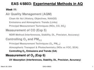
EAS 4/8803: Experimental Methods in AQ Week 11: Air Quality Management (AQM) Clean Air Act (History, Objectives, NAAQS) Emissions and Atmospheric Trends (Links) Principal Measurement Techniques (NOx, CO, SO2) Measurement of CO (Exp 5) NDIR Method (Interferences, Stability, DL, Precision, Accuracy) Controlling O3 and PM2.5 Principal Measurement Techniques (O3, PM2.5) Atmospheric Transport & Photochemistry (NOx vs VOC, SOA) Controlling O3, Emissions and Trends (GA) Measurement of O3 (Exp 6) UV Absorption (Interferences, Stability, DL, Precision, Accuracy) EAS 4/8803
Can we expect recent cool & wet summers to continue? Nonattain “Bad” NAAQS Attain “Good” EAS 4/8803
If we can’t depend on theweather, then what canwe control? Volatile Organic Compounds (VOCs) + Nitrogen Oxides (NOx) Ozone (O3) Smog Combustion Processes Fuels, Paints, Solvents, & Vegetation EAS 4/8803
Photochemical Processes Leading to O3 and PM An Assessment of Tropospheric Ozone Pollution, A North American Perspective, NARSTO, National Acad. Press, 2000. NOz SOA EAS 4/8803
VOC Sources in Columbus MSA (2000) Total: 385 tons per day • Anthropogenic Sources: • Gasoline Vehicles • Solvents (Paints, Automotive Products, Adhesives, etc.) • Carbon Black • Lawn & Garden • Bakeries EAS 4/8803
Ozone Isopleths Area of effective VOC control (most often highly populated areas) Constant [O3] NOx control effective(areas with high biogenics) Nitrogen Oxides (NOx) High [O3] Low [O3] Volatile Organic Compounds (VOC) EAS 4/8803
Total: 42 tons per day NOx Sources in Columbus MSA (2000) EAS 4/8803
Implementation of NOx Controls Since 2000,Full Implementation Expected by 2007 • Annual, stricter vehicle emissions inspections • Open burning ban in 45 counties • Georgia Power phasing in NOx controls • 30 ppm sulfur gasoline in 45 counties • GA Power plants achieve NOx reduction in 45 counties • Stricter peaking generator rule • Large industrial source NOx reductions EAS 4/8803
2007 NOx Emissions in GA by Region and Source If Fully Implemented Georgia Total: 1480 tons/day Alabama Total (not shown): 998 tons/day EAS 4/8803
Significant improvements in regional air quality by 2007with no additional controls (current SIP fully implemented) EAS 4/8803
But will these existing controls be enough? Region Maximum Daily Peak 8-hour Ozone Observed / Simulated 2000 2007 Estimated Change in Regional Peak 8-hour Surface Ozone from August 17th, 2000 to 2007 under the Existing Federal Control Strategies (ppbv) EAS 4/8803
Nonattain “Bad” NAAQS Attain “Good” EAS 4/8803
Nonattain “Bad” NAAQS Attain “Good” Reality Goal Theory EAS 4/8803
COspan4 5 V COspan3 COspan2 D[COnom]4 CO Analyzer Signal (V) D[COnom]3 zero-mode zero-mode COspan1 D[COnom]2 D[COnom]1 COZA COZA Zero-air COspan1,0 COspan4,0 Zero-air/Zero-mode = baseline CO0 CO0 Time (minutes) Clarification CO Accuracy Assessment COsensi (ppb/V) = D[COnomi] / DCOspani ZTeffi = (COspani – COspani,0) / (COspani – CO0) > 0.9!! COnet (V) = COraw – CO0ipol CO (ppb) = COnet * COsens DL (ppb) = t * STD(CO0*) * COsens P (%) = t * STD(COsens) / AVG(COsens) *100 A1 (%) = (slope{D[COnomi] / DCOspani} -1000)/1000 *100 Rel. diff. of slope to nom. detector sens = 1000 ppb/V A2 (%) = {S[(s(Xj))2 (dCOsens/dXj)2]}1/2 …from error propagation analysis. EAS 4/8803
O3 Method: UV Absorption I = I0 e-e c l e = 308 cm-1(@STP: 0oC, 760Torr) l = 38 cm 254 nm EAS 4/8803
To analyzer under cal internal vent [O3]nomC capped Zero Air 254 nm O3 Primary Standard Calibrator I = I0 e-e c l e = 308 cm-1(@STP: 0oC, 760Torr) l = 38 cm EAS 4/8803
Goals • Basic Functionality Test • Determine Analyzer Performance (DL, sensitivity, precision and accuracy) • Determine the NO2 Photolysis Rate from PSS assumptions and discuss • Discuss differences in O3 measured between outdoor and indoor air EAS 4/8803
1. Functionality Tests • Detectors Performance check • System Leaks and Pump check • Ozone scrubber efficiency check EAS 4/8803
O3span1 10 V O3span2 O3span3 D[O3nom]1 O3 Analyzer Signal (V) D[O3nom]2 O3span4 D[O3nom]3 D[O3nom]4 O30 O30 Zero-air Time (minutes) 2. Analyzer Performance O3sensi (ppb/V) = D[O3nomi] / DO3spani O3 (ppb) = O3raw * O3sens DL1 (ppb) = t * STD(O30) * O3sens DL2 (ppb) = i-cept{D[O3nomi] / DO3spani} P (%) = t * STD(O3sensi) / AVG(O3sensi) *100 A1 (%) = (slope{D[O3nomi] / DO3spani} -20)/20 *100 Rel. diff. of slope to nom. detector sens = 20 ppb/V A2 (%) = {S[(s(Xj))2 (dO3sens/dXj)2]}1/2 …from error propagation analysis. Groups look for their individual “O3raw__.xls” data file on http://arec.gatech.edu/teaching EAS 4/8803
3.1 Determine jNO2 from PSS Assuming ambient O3 in photochemical steady-state (PSS) with NO and NO2, calculate jNO2 and discuss by comparing with literature values. NO2 + hv (jNO2) NO + O (R1) O + O2 + M O3 + M (fast, not rate-limiting) (R2) O3 + NO (k3) NO2 + O2 (R3) Assuming first-order homogeneous reaction (R3),and d[NO2]/dt = k3 [O3][NO] - jNO2 [NO2] = 0 yielding jNO2 = k3 [NO] [O3] / [NO2] in s-1 EAS 4/8803
3.2 Discuss jNO2 Diurnal Profile The photolysis rate coefficients (jNO2) provided here exemplarily, were calculated using a radiative transfer model (Zeng et al., 1996), which is based upon the Stamnes discrete ordinates model modified to solve the radiative transfer equation in pseudo-spherical coordinates. The discrete ordinates code was run with eight streams. The surface albedo was assumed to be 5%, and the total aerosol optical depth was parameterized in terms of visual range. The model assumes a constant visual range of 25 km for the lowest 2 km, a logarithmically decreasing aerosol optical depth above this, as well as a single scattering albedo of 0.99 and an asymmetry parameter of 0.61, which are both wavelength-independent. The jNO2 values were then scaled linearly by the flat-plate Eppley-UV (290-385 nm) measurements and by their ratio to the radiative transfer model clear-sky irradiance to account for the actual cloud and aerosol effects on jNO2. This scaling helps to correct for any errors made by the visual range assumptions. Consult references Volz et al., 1996, and Zeng et al., 1996. Retrieve above sample data as “jNO2sampleday.xls” from http://arec.gatech.edu/teaching EAS 4/8803
4. Discuss O3 indoor vs outdoor differences • Determine indoor and outdoor O3 mixing ratios for a sample data set. • Evaluate diurnal profiles of both individually and as difference. • Discuss observed differences. Look for “O3inoutday.xls” At http://arec.gatech.edu/teaching EAS 4/8803