Download
1 / 16
160 likes | 253 Views
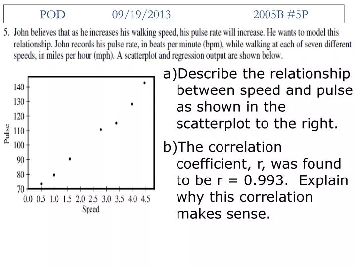
POD 09/19/2013 2005B #5P. Describe the relationship between speed and pulse as shown in the scatterplot to the right. The correlation coefficient, r, was found to be r = 0.993. Explain why this correlation makes sense. Linear Regression. AP Statistics Chapter 8 Day 1.

E N D
POD 09/19/2013 2005B #5P • Describe the relationship between speed and pulse as shown in the scatterplot to the right. • The correlation coefficient, r, was found to be r = 0.993. Explain why this correlation makes sense.
Linear Regression AP Statistics Chapter 8 Day 1
Learning Targets What is the LSRL? Why do we compute the LSRL? How do we use formulas to compute the LSRL?
What does “Least Squares” Mean? The “Line of Best Fit” – called the LSRL is the line that minimizes the sum of the squared errors The “error” (distance the data point is from the line is called a residual. Residual = Actual – Predicted
LSRL (linear model) • Least squares regression line of y on x is the line that makes the sum of the squares of the vertical distances of the data points from the line as small as possible. Line of Best Fit!
Y-hat is the predicted response • As correlation grows weaker, the prediction y-hat moves less in response to changes in x. (prediction gets worse!) • Conditions are the same as correlation
Steps for Regression • Identify the variables and check the conditions (always look at the scatterplot) • Report summary statistics for x and y (mean and std. deviation) • Find the slope, b1. • Find the intercept, b0. • Write the regression equation using the variable names. • Conclusion: interpret the equation in context.
Interpreting slope: For every increase in __x__, the model predicts on average an __inc/dec__ of slope value units in ___y___.
Interpreting the Y-intercept… In General Y-Intercept: When x-variable is zero, the y-variable is predicted to be y-intercept value. *** Note: this value does not always make sense!!
Find the LSRL X-values: Mean = 10, St Dev = 2 Y-values: Mean = 20, St Dev = 3 r = 0.5 Slope: Y-intercept: Equation:
The following data is on x= age in years and y = weight in kg for 12 black bears. • Find the LSRL using the formulas. • Interpret the slope of the LSRL.
Verbal SAT vs Math SAT V: mean=596.3 st.dev=99.5 M: mean=612.2 st.dev=96.1 r = 0.685 Write the equation of the LSRL Interpret the slope of this line Interpret the intercept of this line. Slope = 0.685(96.1/99.5) = 0.662 Y-int = 612.2 – (0.662*596.3) =217.45 Math SAT = 217.45 + 0.662 (Verbal SAT) For every point on the Verbal SAT, your Math SAT increases by approx 0.662 pts If you get a zero Verbal score, you are predicted to get a 217.45 on the Math
Homework • P. 192 # 1, 5, 7, 36