Download
1 / 23
230 likes | 401 Views
When one neuron contributes to the firing of another neuron the pathway between them is strengthened. That is, if the output of i is the input to j, then the weight is adjusted by a quantity proportional to c * (o i * o j). Hebbian Coincidence Learning. The rule is Δ W = c * f(X,W) * X

E N D
When one neuron contributes to the firing of another neuron the pathway between them is strengthened. That is, if the output of i is the input to j, then the weight is adjusted by a quantity proportional to c * (oi * oj). Hebbian Coincidence Learning
The rule is ΔW = c * f(X,W) * X An example of unsupervised Hebbian learning is to simulate transfer of a response from a primary or unconditioned stimulus to a conditioned stimulus. Unsupervised Hebbian Learning
In this example, the first three inputs represented the unconditioned stimuli and the second three inputs represent the new stimuli. Example (cont'd)
In supervised Hebbian learning, instead of using the output of a neuron, we use the desired output as supplied by the instructor. The rule becomes ΔW = c * D * X Supervised Hebbian Learning
Recognizing associations between sets of patterns: {<X1, Y1>, <X2, Y2>, ... <Xt, Yt>}. The input to the network would be pattern Xi and the output should be the associated pattern Yi. The network consists on an input layer with n neurons (where n is the number of different input patterns, and with an output layer of size m, where m is the number of output pattens. The network is fully connected. Example
In this example, the learning rule becomes: ΔW = c * Y * X, where Y * X is the outer vector product. We cycle through the pairs in the training set, adjusting the weights each time This kind of network (one the maps input vectors to output vectors using this rule) is called a linear associator. Example (cont'd)
Used for memory retrieval, returning one pattern given another. There are three types of associative memory Heteroassociative: Mapping from X to Y s.t. if an arbitrary vector is closer to Xi than to any other Xj, the vector Yi associated with Xi is returned. Autoassociative: Same as above except that Xi = Yi for all exemplar pairs. Useful in retrieving a full pattern from a degraded one. Associative Memory
Interpolative: If X differs from the exemplar Xi by an amount Δ, then the retrieved vector Y differs from Yi by some function of Δ. A linear associative network (one input layer, one output layer, fully connected) can be used to implement interpolative memory. Associative Memory (cont'd)
Hamming vectors are vectors composed of just the numbers +1 and -1. Assume all vectors are size n. The Hamming distance between two vectors is just the number of components which differ. An orthonormal set of vectors is a set of vectors where are all unit length and each pair of distinct vectors is orthogonal (the cross-product of the vectors is 0). Representation of Vectors
If the input set of vectors is orthonormal, then a linear associative network implements interpolative memory. The output is the weighted sum of the input vectors (we assume a trained network). If the input pattern matches one of the exemplars, Xi, then the output will be Yi. If the input pattern is Xi + Δi, then the output will be Yi + Φ(Δi) where Φ is the mapping function of the network. Properties of a LAN
If the exemplars do not form an orthonormal set, then there may be interference between the stored patterns. This is know as crosstalk. The number of patterns which may be stored is limited by the dimensionality of the vector space. The mapping from real-life situations to orthonormal sets may not be clear. Problems with LANs
Instead of return an interpolation, we may wish to return the vector associated with closest exemplar. We can create such a network (an attactor network) by using feedback instead of a strictly feed-foward network. Attractor Network
Feedback networks have the following properties: There are feedback connections between the nodes This is a time delay in signal, i.e., signal propagation is no instantaneous The output of the network depends on the network state upon convergence of the signals. Usefulness depends on convergence Feedback Network
A feedback network is initialized with an input pattern. The network then processes the input, passing signal between nodes, going through various states until it (hopefully) reaches equilibrium. The equilibrium state of the network supplies the output. Feedback networks can be used for heteroassociative and autoassociative memories. Feedback Network (cont'd)
An attractor is a state toward which other states in the region evolve in time. The region associated with an attractor is called a basin. Attractors
A bi-directional associative memory (BAM) network is one with two fully connected layers, in which the links are all bi-directional. There can also be a feedback link connecting a node to itself. A BAM network may be trained, or its weights may be worked out in advance. It is used to map a set of vectors Xi (input layer) to a set of vectors Yi (output layer). Bi-Directional Associative Memory
If a BAM network is used to implement an autoassocative memory then the input layer is the same as the output layer, i.e., there is just one layer with feedback links connecting nodes to themselves in addition to the links between nodes. This network can be used to retrieve a pattern given a noisy or incomplete pattern. BAM for autoassociative memory
Apply an initial vector pair (X,Y) to the processing elements. X is the pattern we wish to retrieve and Y is random. Propagate the information from the X layer to the Y layer and update the values at the Y layer. Send the information back to the X layer, updating those nodes. Continue until equilibrium is reached. BAM Processing
Two goals: Guarantee that the network converges to a stable state, no matter what input is given. The stable state should be the closest one to the input state according to some distance metric Hopfield Networks
A Hopfield Network is identical in structure to an autoassociative BAM network – one layer of fully connected neurons. The activation function is +1, if net > Ti, xnew = xold, if net = Ti, -1, if net < Ti, where net = Σj wj * xj. Hopfield Network (cont'd)
The are restrictions on the weights: wii = 0 for all i, and wij = wji for i.j. Usually the weights are calculated in advance, rather than having the net trained. The behavior of the net is characterized as an energy function, H(X) = - Σi Σj wij wi wj + 2 Σi Ti xi, decreases from every network transition. More on Hopfield Nets
Thus, the network must converge, and converge to a local energy minimum, but there is no guarantee that in converges to a state near the input state. Can be used for optimization problems such a TSP (map the cost function of the optimization problem to the energy function of the Hopfield net). Hopfield Nets