Download
1 / 29
290 likes | 441 Views
几种常见的优化方法. 电子结构 几何机构. 稳定点 最小点. 函数. Taylor 展开: V(x) = V(x k ) + (x-x k )V’(x k ) +1/2 (x-x k ) 2 V’’(x k )+…. 当 x 是 3N 个变量的时候, V’(x k ) 成为 3Nx1 的向量,而 V’’(x k ) 成为 3Nx3N 的矩阵,矩阵元如:. Hessian. 一阶梯度法 a. Steepest descendent. 最速下降法. S k = -g k /|g k |. direction. gradient.

E N D
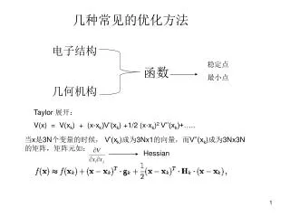
几种常见的优化方法 电子结构 几何机构 稳定点 最小点 函数 Taylor 展开: V(x) = V(xk) + (x-xk)V’(xk) +1/2 (x-xk)2 V’’(xk)+….. 当x是3N个变量的时候, V’(xk)成为3Nx1的向量,而V’’(xk)成为3Nx3N的矩阵,矩阵元如: Hessian
一阶梯度法 • a. Steepest descendent 最速下降法 Sk = -gk/|gk| direction gradient 知道了方向,如何确定步长呢? 最常用的是先选择任意步长l,然后在计算中调节 用体系的能量作为外界衡量标准,能量升高了则逐步减小步长。 robust, but slow
b. Conjugate Gradient (CG) 共轭梯度 不需要外界能量等作为衡量量 利用了上一步的信息 第k步的方向 标量 Usually more efficient than SD, also robust
2。二阶梯度方法 牛顿-拉夫逊法 这类方法很多,最简单的称为Newton-Raphson方法, 而最常用的是Quasi-Newton方法。 Quasi-Newton方法: use an approximation of the inverse Hessian. Form of approximation differs among methods Broyden-Fletcher-Golfarb-Shanno BFGS method DFP method Davidon-Fletcher-Powell
Molecular dynamics 分子动力学 History It was not until 1964 that MD was used to study a realistic molecular system, in which the atoms interacted via a Lennard-Jones potential. After this point, MD techniques developed rapidly to encompass diatomic species, water (which is still the subject of current research today!), small rigid molecules, flexible hydrocarbons and now even macromolecules such as proteins and DNA. These are all examples of continuous dynamical simulations, and the way in which the atomic motion is calculated is quite different from that in impulsive simulations containing hard-core repulsions.
What can we do with MD – Calculate equilibrium configurational properties in a similar fashion to MC. – Study transport properties (e.g. mean-squared displacement and diffusion coefficients). Extend the basic MD algorithm – MD in the NVT, NpT and NpH ensembles – The united atom approximation – Constraint dynamics and SHAKE – Rigid body dynamics – Multiple time step algorithms
‘Impulsive’ molecular dynamics 1.Dynamics of perfectly ‘hard’ particles can be solved exactly, but process becomes involved for many part (N-body problem). 2.Can use a numerical scheme that advances the system forward in time until a collision occurs. 3.Velocities of colliding particles (usually a pair!) then recalculated and system put into motion again. 4. Simulation proceeds by fits and starts, with a mean time between collisions related to the average kinetic energy of the particles. 5.Potentially very efficient algorithm, but collisions between particles of complex shape are not easy to solve, and cannot be generalised to continuous potentials.
Continuous time molecular dynamics 1. By calculating the derivative of a macromolecular force field, we can find the forces on each atom as a function of its position. 2. Require a method of evolving the positions of the particles in space and time to produce a ‘true’ dynamical trajectory. 3. Standard technique is to solve Newton’s equations of motion numerically, using some finite difference scheme, which is known as integration. 4. This means that we advance the system by some small time step Δt, recalculate the forces and velocities, and then repeat the process iteratively. 5. Provided Δt is small enough, this produces an acceptable approximate solution to the continuous equations of motion.
Example of integrator for MD simulation • One of the most popular and widely used integrators is • the Verlet leapfrog method: positions and velocities of • particles are successively ‘leap-frogged’ over each other • using accelerations calculated from force field. • The Verlet scheme has the advantage of high precision • (of order Δt4), which means that a longer time step can • be used for a given level of fluctuations. • The method also enjoys very low drift, provided an • appropriate time step and force cut-off are used. r(t+Dt)=r(t)+v(t+Dt/2)Dt v(t+Dt/2)=v(t-Dt/2)+a(t+Dt/2)Dt
Other integrators for MD simulations • Although the Verlet leapfrog method is not particularly • fast, this is relatively unimportant because the time • required for integration is usually trivial in comparison to • the time required for the force calculations. • The most important concern for an integrator is that it • exhibits low drift, i.e. that the total energy fluctuates about • some constant value. A necessary (but not sufficient) • condition for this is that it is symplectic. • Crudely speaking, this means that it should be time • reversible (like Newton’s equations), i.e. if we reverse the • momenta of all particles at a given instant, the system • should trace back along its previous trajectory.
Other integrators for MD simulations • The Verlet method is symplectic, but methods such as • predictor-corrector schemes are not. • Non-symplectic methods generally have problems with • long term energy conservation. • Having achieved low drift, would also like the energy • fluctuations for a given time step to be as low as possible. • Always desirable to use the largest time step possible. • In general, the trajectories produced by integration will • diverge exponentially from their true continuous paths due • to the Lyapunov instability. • However, this does not concern us greatly, as the thermal • sampling is unaffected ⇒ expectation values unchanged.
Choosing the correct time step… 1.The choice of time step is crucial: too short and phase space is sampled inefficiently, too long and the energy will fluctuate wildly and the simulation may become catastrophically unstable (“blow up”). 2. The instabilities are caused by the motion of atoms being extrapolated into regions where the potential energy is prohibitively high (e.g. atoms overlapping). 3. A good rule of thumb is that when simulating an atomic fluid, the time step should be comparable to the mean time between collisions (about 5 fs for Ar at 298K). 4. For flexible molecules, the time step should be an order of magnitude less than the period of the fastest motion (usually bond stretching: C—H around 10 fs so use 1 fs).
For classic MD, there could be many tricks to speed up calculations, all centering around reducing the effort involved in the calculation of the interatomic forces, as this is generally much more time-consuming than integration. • For example • Truncate the long-range forces: charge-charge, charge-dipole • Look-up tables For first principles MD, as forces are evaluated from quantum mechanics, we are only concerned with the time-step.
The simplest MD, like verlet method, is a deterministic simulation technique for evolving systems to equilibrium by solving Newton’s laws numerically. Because the interactions are completely elastic and pairwise acting, both energy and momentum are conserved. Therefore, MD naturally samples from the microcanonical or NVE ensemble. As mentioned previously, the NVE ensemble is not very useful for studying real systems. We would like to be able to simulate systems at constant temperature or constant pressure.
MD in different thermodynamic ensembles • In this lecture, we will discuss ways of using MD to • sample from different thermodynamic ensembles, which • are identified by their conserved quantities. • Canonical (NVT) • – Fixed number of particles, total volume and temperature. • Requires the particles to interact with a thermostat. • Isobaric-isothermal (NpT) • – Fixed number of particles, pressure and temperature. Requires • particles to interact with a thermostat and barostat. • Isobaric-isenthalpic (NpH) • – Fixed number of particles, pressure and enthalpy. Unusual, but • requires particles to interact with a barostat only.
Advanced applications of MD • We will then study some more advanced MD methods • that are designed specifically to speed up, or make • possible, the simulation of large scale macromolecular • systems. • All these methods share a common principle: they freeze • out, or decouple, the high frequency degrees of freedom. • This enables the use of a larger time step without • numerical instability. • These methods include: • – United atom approximation • – Constraint dynamics and SHAKE • – Rigid body dynamics • – Multiple time step algorithms
Revision of NVE MD • Let’s start by revising how to do NVE MD. • Recall that we calculated the forces on all atoms from the • derivative of the force field, then integrated the e.o.m. • using a finite difference scheme with some time step Δt. • We then recalculated the forces on the atoms, and • repeated the process to generate a dynamical trajectory • in the NVE ensemble. • Because the mean kinetic energy is constant, the average • kinetic temperature TK is also constant. • However, in thermal equilibrium, we know that • instantaneous TK will fluctuate. If we want to sample from • the NVT ensemble, we should keep the statistical • temperature constant.
Extended Lagrangians • There are essentially two ways to keep the statistical • temperature constant, and therefore sample from the true • NVT ensemble. • – Stochastically, using hybrid MC/MD methods • – Dynamically, via an extended Lagrangian • We will describe the latter method in this lecture • An extended Lagrangian is simply a way of including a • degree of freedom which represents the reservoir, and • then carrying out a simulation on this extended system. • Energy can flow dynamically back and forth from the • reservoir, which has a certain thermal ‘inertia’ associated • with it. All we have to do is add some terms to Newton’s • equations of motion for the system.
Extended Lagrangians • The standard Lagrangian L is written as the difference of • the kinetic and potential energies: • Newton’s laws then follow by substituting this into the • Euler-Lagrange equation: • Newton’s equations and Lagrangian formalism are • equivalent, but the latter uses generalised coordinates. . .
Canonical MD • So, our extended Lagrangian includes an extra • coordinate ζ, which is a frictional coefficient that evolves in time so as to minimise the difference between the instantaneous kinetic and statistical temperatures. • The modified equations of motion are: • The conserved quantity is the Helmholtz free energy. (modified form of Newton II)
Canonical MD • By adjusting the thermostat relaxation time tT(usually • in the range 0.5 to 2 ps) the simulation will reach an • equilibrium state with constant statistical temperature TS. • TS is now a parameter of our system, as opposed to the • measured instantaneous value of TK which fluctuates • according to the amount of thermal energy in the system • at any particular time. • Too high a value of tT and energy will flow very slowly • between the system and the reservoir (overdamped). • Too low a value of tT and temperature will oscillate about • its equilibrium value (underdamped). • This is the Nosé-Hoover thermostat method.
Canonical MD • There are many other methods for achieving constant • temperature, but not all of them sample from the true • NVT ensemble due to a lack of microscopic reversibility. • We call these pseudo-NVT methods, and they include: • – Berendsen method • Velocities are rescaled deterministically after each step so that the system is forced towards the desired temperature • – Gaussian constraints • Makes the kinetic energy a constant of the motion by minimising the least squares difference between the Newtonian and constrained trajectories • These methods are often faster, but only converge on the • true canonical average properties as O(1/N).
Isothermal-isobaric MD • We can apply the extended Lagrangian approach to simulations at constant pressure by simply adding yet another coordinate to our system. • We use η, which is a frictional coefficient that evolves in • time to minimise the difference between the instantaneous pressure p(t), measured by a virial expression, and the pressure of an external reservoir pext. • The equations of motion for the system can then be obtained by substituting the modified Lagrangian into the Euler-Lagrange equations. • These now include two relaxation times: one for the • thermostat tT, and one for the barostat tp.
Isothermal-isobaric MD The is known as the Nosé-Hoover method (Melchionna type) and the equations of motion are:
Constraint dynamics freeze the bond stretching motions of the hydrogens (or any other bond, in principle). • We apply a set of holonomic constraints to the system, which are just algebraic equations connecting the coordinates of the individual atoms. These constraints contain information about the bond lengths. • The most widely used algorithm for implementing these constraints is called SHAKE. This works on the principle of applying fictitious forces to all the particles such that they follow appropriately constrained trajectories. • There is also a variant of SHAKE called RATTLE.
We can calculate what the constraint forces are (obviously they must be directed parallel to the bonds) by introducing Lagrange multipliers lij: These multipliers can be determined by substituting the modified expressions for Newton II into our Verlet integration scheme and imposing the constraints that:
This leads to a set of simultaneous equations for lijwhich • can be recast into a matrix form and solved by inverting • the matrix. • For larger molecules, this is very time consuming and so • an iterative procedure is used (hence the “shaking” of the • molecule as each constraint is enforced in turn). • Angle and higher order constraints can easily be • incorporated into the algorithm by enforcing fictitious • constraint bonds between atoms such that the angle • between them is held constant. • However, there are problems with convergence of the • algorithm if the molecule is overconstrained.