Demand Forecasting

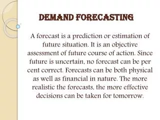
1. Demand Forecasting EMBA 512 Demand Forecasting Boise State University

2. Objectives • Understand the role of forecasting • Understand the issues • Understand basic tools and techniques EMBA 512 Demand Forecasting Boise State University

3. Forecasting • Developing predictions or estimates of future values • Demand volume • Price levels • Lead times • Resource availability • ... EMBA 512 Demand Forecasting Boise State University

4. The Role of Forecasting • Necessary Input to all Planning Decisions • Operations: Inventory, Production Planning & Scheduling • Finance: Plant Investment & Budgeting • Marketing: Sales-Force Allocation, Pricing Promotions • Human Resources: Workforce Planning EMBA 512 Demand Forecasting Boise State University

5. Demand Forecasting For manufactured items and conventional goods, forecasts are used to determine • Replenishment levels and safety stocks • Set production plans • Determine procurement schedules • Capacity planning, financial planning, & workforce planning EMBA 512 Demand Forecasting Boise State University

6. Demand Forecasting For services, demand forecasts are used for • Capacity planning, workforce scheduling, procurement & budgeting. • Because services cannot be stored, demand forecasting for services is often concerned with forecasting the peak demand, rather than the average demand and its range. EMBA 512 Demand Forecasting Boise State University

7. Characteristics of Forecasts • Forecast are always wrong. A good forecast is more than a single value. • Forecast accuracy decreases with the forecast horizon. • Aggregate forecasts are more accurate than disaggregated forecasts. EMBA 512 Demand Forecasting Boise State University

8. Independent vs. Dependent Demand • Independent • Exogenously controlled • Subject to random or unpredictable changes • What we forecast • Dependent or Derived • Calculated or derived from other sources • Do not forecast EMBA 512 Demand Forecasting Boise State University

9. Forecasting Methods Qualitative or Judgmental • Ask people who ought to know • Historical Projection or Extrapolation • Time Series Models • Moving Averages • Exponential Smoothing • Regression based methods EMBA 512 Demand Forecasting Boise State University

10. Basic Approach to Demand Forecasting • Identify the Objective of the Forecast • Integrate Forecasting with Planning • Identify the Factors that Influence the Demand Forecast • Identify the Appropriate Forecasting Model • Monitor the Forecast (Measure Errors) EMBA 512 Demand Forecasting Boise State University

11. Time Series Methods • Appropriate when future demand is expected to follow past demand patterns. • Future demand is assumed to be influenced by the current demand, as well as historical growth and seasonal patterns. EMBA 512 Demand Forecasting Boise State University

12. Time Series Models With time series models observed demand can be broken down into two components: systematic and random. Observed Demand = Systematic Component + Random Component EMBA 512 Demand Forecasting Boise State University

13. Time Series Methods The systematic component is the expected demand value. It is comprised of the underlying average demand, the trend in demand, and the seasonal fluctuations (seasonality) in demand. EMBA 512 Demand Forecasting Boise State University

14. Idea Behind Time Series Models Distinguish between random fluctuations and true changes in underlying demand patterns. EMBA 512 Demand Forecasting Boise State University

15. Time Series Components of Demand Demand Random component Time EMBA 512 Demand Forecasting Boise State University

16. Monthly chart of the DJIA's changes from month to month along with a 3 period simple moving average. EMBA 512 Demand Forecasting Boise State University

17. Time Series Methods • The random component cannot be predicted. However, its size and variability can be estimated to provide a measure of forecast error. The objective of forecasting is to filter the random component and model (estimate) the systematic component. EMBA 512 Demand Forecasting Boise State University

18. Moving Averages • Simple, widely used • Reduce random noise • One Extreme • Prediction next period = Demand this period • Another Extreme • Prediction next period = Long run average • Intermediate View • Prediction next period = Average of last n periods EMBA 512 Demand Forecasting Boise State University

19. Period Demand 1 12 2 15 3 11 4 9 5 10 6 8 7 14 8 12 Moving Average Models  3-period moving average forecast for Period 8: = (14 + 8 + 10) / 3 = 10.67 EMBA 512 Demand Forecasting Boise State University

20. Weighted Moving Averages Forecast for Period 8 = [(0.5 14) + (0.3 8) + (0.2 10)] / (0.5 + 0.3 + 0.2) = 11.4 What are the advantages? What do the weights add up to? Could we use different weights? Compare with a simple 3-period moving average. EMBA 512 Demand Forecasting Boise State University

21. Table of Forecasts and Demand Values . . . EMBA 512 Demand Forecasting Boise State University

22. . . . and Resulting Graph Note how the forecasts smooth out variations EMBA 512 Demand Forecasting Boise State University

23. Simple Exponential Smoothing • Sophisticated weighted averaging model • Needs only three numbers: Ft = Forecast for the current period tDt = Actual demand for the current period t a = Weight between 0 and 1 EMBA 512 Demand Forecasting Boise State University

24. Exponential Smoothing • Moving Averages • Equal weight to older observations • Exponential Smoothing • More weight to more recent observations • Forecast for next period is a weighted average of • Observation for this period • Forecast for this period EMBA 512 Demand Forecasting Boise State University

25. Simple Exponential Smoothing Formula Ft+1 = Ft + a (Dt – Ft) = a ×Dt + (1 – a) × Ft • Where did the current forecast come from? • What happens as a gets closer to 0 or 1? • Where does the very first forecast come from? EMBA 512 Demand Forecasting Boise State University

26. Exponential Smoothing Forecast with a = 0.3 F2 = 0.3×12 + 0.7×11 = 3.6 + 7.7 = 11.3 F3 = 0.3×15 + 0.7×11.3 = 12.41 EMBA 512 Demand Forecasting Boise State University

27. Resulting Graph EMBA 512 Demand Forecasting Boise State University

28. Time Series with Demand random and trend components Time EMBA 512 Demand Forecasting Boise State University

29. Linear Trend EMBA 512 Demand Forecasting Boise State University

30. Exponential Trend EMBA 512 Demand Forecasting Boise State University

31. Trends What do you think will happen to a moving average or exponential smoothing model when there is a trend in the data? EMBA 512 Demand Forecasting Boise State University

32. Simple Exponential Smoothing Always Lags A Trend Because the model is based on historical demand, it always lags the obvious upward trend EMBA 512 Demand Forecasting Boise State University

33. SimpleLinear Regression • Time Series • Find best fit of proposed model to past data • Project that fit forward • Assumes a linear relationship: y = a + b(x) y x EMBA 512 Demand Forecasting Boise State University

34. Definitions Y = a + b(X) Y = predicted variable (i.e., demand) X = predictor variable “X” is the time period for linear trend models. EMBA 512 Demand Forecasting Boise State University

35. Example:Regression Used to Estimate A Linear Trend Line EMBA 512 Demand Forecasting Boise State University

36. Resulting Regression Model:Forecast = 10 + 98×Period EMBA 512 Demand Forecasting Boise State University

37. Time series with Demand random, trend and seasonal components June June June June EMBA 512 Demand Forecasting Boise State University

38. Trend & Seasonality EMBA 512 Demand Forecasting Boise State University

39. Seasonality EMBA 512 Demand Forecasting Boise State University

40. Modeling Trend & Seasonal Components Quarter Period Demand Winter 07 1 80 Spring 2 240 Summer 3 300 Fall 4 440 Winter 08 5 400 Spring 6 720 Summer 7 700 Fall 8 880 EMBA 512 Demand Forecasting Boise State University

41. What Do You Notice? EMBA 512 Demand Forecasting Boise State University

42. Regression picks up trend, butnot the seasonality effect EMBA 512 Demand Forecasting Boise State University

43. Calculating Seasonal Index: Winter Quarter (Actual / Forecast) for Winter Quarters: Winter ‘07: (80 / 90) = 0.89 Winter ‘08: (400 / 524.3) = 0.76 Average of these two = 0.83 Interpret! EMBA 512 Demand Forecasting Boise State University

44. Seasonally Adjusted Forecast Model For Winter Quarter [ –18.57 + 108.57×Period ] × 0.83 Or more generally: [ –18.57 + 108.57 × Period ] ×Seasonal Index EMBA 512 Demand Forecasting Boise State University

45. Seasonally Adjusted Forecasts EMBA 512 Demand Forecasting Boise State University

46. Would You Expect the Forecast Model to Perform This Well With Future Data? EMBA 512 Demand Forecasting Boise State University

47. The Perfect (Imaginary) Forecast EMBA 512 Demand Forecasting Boise State University

48. A More Realistic Forecast EMBA 512 Demand Forecasting Boise State University

49. Forecast Error • Building a Forecast • Fit to historical data • Project future data • Forecast Error • How well does model fit historical data • Do we need to tune or refine the model • Can we offer confidence intervals about our predictions EMBA 512 Demand Forecasting Boise State University

50. Forecast Error • The forecast error measures the difference between the actual demand and the forecast of demand. The forecast is based on the systematic component and the random component is estimated based on the forecast error. • Forecast Error = Actual – Forecast EMBA 512 Demand Forecasting Boise State University