Download
1 / 55
550 likes | 851 Views
Motion Planning. Howie CHoset. Assign HW. Algorithms. Start-Goal Methods Map-Based Approaches Cellular Decompositions. Motion Planning Statement. If W denotes the robot’s workspace, And C i denotes the i’th obstacle, Then the robot’s free space, FS, is defined as:

E N D
Motion Planning Howie CHoset
Algorithms • Start-Goal Methods • Map-Based Approaches • Cellular Decompositions
Motion Planning Statement If W denotes the robot’s workspace, And Cidenotes the i’th obstacle, Then the robot’s free space, FS, is defined as: FS = W - ( U Ci ) And a path c C0is c : [0,1] g FS where c(0) is qstart and c(1) is qgoal
What if the robot is not a point? The Scout should probably not be modeled as a point... b a Nor should robots with extended linkages that may contact obstacles...
Configuration Space “Quiz” Where do we put ? 360 qA A 270 b B 180 b 90 a qB a 0 45 135 90 180 An obstacle in the robot’s workspace Torus (wraps horizontally and vertically)
Configuration Space Obstacle How do we get from A to B ? Reference configuration 360 qA A 270 b B 180 b 90 a qB a 0 45 135 90 180 An obstacle in the robot’s workspace The C-space representation of this obstacle…
Two Link Path Thanks to Ken Goldberg
Map-Based Approaches: Roadmap Theory • Properties of a roadmap: • Accessibility: there exists a collision-free path from the start to the road map • Departability: there exists a collision-free path from the roadmap to the goal. • Connectivity: there exists a collision-free path from the start to the goal (on the roadmap). • a roadmap exists a path exists • Examples of Roadmaps • Generalized Voronoi Graph (GVG) • Visibility Graph
Roadmap: Visibility Graph • Formed by connecting all “visible” vertices, the start point and the end point, to each other • For two points to be “visible” no obstacle can exist between them • Paths exist on the perimeter of obstacles • In our example, this produces the shortest path with respect to the L2 metric. However, the close proximity of paths to obstacles makes it dangerous
The Visibility Graph in Action (Part 1) • First, draw lines of sight from the start and goal to all “visible” vertices and corners of the world. goal start
The Visibility Graph in Action (Part 2) • Second, draw lines of sight from every vertex of every obstacle like before. Remember lines along edges are also lines of sight. goal start
The Visibility Graph in Action (Part 3) • Second, draw lines of sight from every vertex of every obstacle like before. Remember lines along edges are also lines of sight. goal start
The Visibility Graph in Action (Part 4) • Second, draw lines of sight from every vertex of every obstacle like before. Remember lines along edges are also lines of sight. goal start
The Visibility Graph (Done) • Repeat until you’re done. goal start
Visibility Graph Overview • Start with a map of the world, draw lines of sight from the start and goal to every “corner” of the world and vertex of the obstacles, not cutting through any obstacles. • Draw lines of sight from every vertex of every obstacle like above. Lines along edges of obstacles are lines of sight too, since they don’t pass through the obstacles. • If the map was in Configuration space, each line potentially represents part of a path from the start to the goal.
Roadmap: GVG • A GVG is formed by paths equidistant from the two closest objects • Remember “spokes”, start and goal • This generates a very safe roadmap which avoids obstacles as much as possible
Two-Equidistant • Two-equidistant surface
SS ij More Rigorous Definition Going through obstacles Two-equidistant face
S ij Two-Equidistant • Two-equidistant surface Two-equidistant surjective surface Two-equidistant Face
Voronoi Diagram (L2) Note the curved edges
Voronoi Diagram (L1) Note the lack of curved edges
Exact Cell vs. Approximate Cell • Cell: simple region
c14 c7 c4 c5 c8 c2 c15 c11 c1 c10 c13 c1 c8 c9 c11 c2 c3 c4 c7 c5 c6 c3 c9 c6 c12 c12 c13 c15 c14 c10 Adjacency Graph • Node correspond to a cell • Edge connects nodes of adjacent cells • Two cells are adjacent if they share a common boundary
Cell Decompositions: Trapezoidal Decomposition • A way to divide the world into smaller regions • Assume a polygonal world
Cell Decompositions: Trapezoidal Decomposition • Simply draw a vertical line from each vertex until you hit an obstacle. This reduces the world to a union of trapezoid-shaped cells
Applications: Coverage • By reducing the world to cells, we’ve essentially abstracted the world to a graph.
Find a path • By reducing the world to cells, we’ve essentially abstracted the world to a graph.
Find a path • With an adjacency graph, a path from start to goal can be found by simple traversal start goal
Find a path • With an adjacency graph, a path from start to goal can be found by simple traversal start goal
Find a path • With an adjacency graph, a path from start to goal can be found by simple traversal start goal
Find a path • With an adjacency graph, a path from start to goal can be found by simple traversal start goal
Find a path • With an adjacency graph, a path from start to goal can be found by simple traversal start goal
Find a path • With an adjacency graph, a path from start to goal can be found by simple traversal start goal
Find a path • With an adjacency graph, a path from start to goal can be found by simple traversal start goal
Find a path • With an adjacency graph, a path from start to goal can be found by simple traversal start goal
Find a path • With an adjacency graph, a path from start to goal can be found by simple traversal start goal
Find a path • With an adjacency graph, a path from start to goal can be found by simple traversal start goal
Find a path • With an adjacency graph, a path from start to goal can be found by simple traversal start goal