Download
1 / 26
260 likes | 363 Views
New Courses in the Fall Biodiversity -- Pennings Evolution of Development -- Azevedo Lab/Field Positions. Dynamics of Unlinked Loci two loci, each on a different chromosome A: A 1 , A 2 f (A 1 ) = p, f (A 2 ) = q B: B 1 , B 2 f (B 1 ) = r, f (B 2 ) = s.

E N D
New Courses in the Fall Biodiversity -- Pennings Evolution of Development -- Azevedo Lab/Field Positions
Dynamics of Unlinked Loci two loci, each on a different chromosome A: A1, A2f (A1) = p, f (A2) = q B: B1, B2f (B1) = r, f (B2) = s Under Hardy-Weinberg Equilibrium, the expected genotype frequencies for each locus are: A: f (A1A1) = p2f (A1A2) = 2pq f (A2A2) = q2 B: f (B1B1) = r2f (B1B2) = 2rs f (B2B2) = s2 If the population is in HWE, the 2-locus genotype frequencies are the joint probabilities: f (A1A1B1B1) = p2r2f (A1A2B1B1) = 2pqr2f (A2A2B1B1) = q2r2 f (A1A1B1B2) = 2rsp2f (A1A2B1B2) = 2pq2rs f (A2A2B1B2) = 2rsq2 f (A1A1B2B2) = p2s2f (A1A2B2B2) = 2pq s2f (A2A2B2B2) = q2s2
Significant Deviation From 2-locus HWE ---> significant non-random association of genotypes = linkage disequilibrium (w/ or w/o physical linkage) measuring the degree of association: use expected vs. observed distribution of gamete types gamete exp. freq. obs. freq. if loci are independent, A1B1 pr a exp. freq. = obs. freq. A1B2 ps b i.e., pr – a = 0, etc. A2B1 qr c A2B2 qs d what if pr – a 0 ?? D / gametic disequilibrium parameter /deviation from random association between alleles D = a – pr; more generally, D = ad - bc
significant deviation from 2-locus HWE ---> significant non-random association of genotypes = linkage disequilibrium (w/ or w/o physical linkage) measuring the degree of association: use expected vs. observed distribution of gamete types gamete exp. freq. obs. freq. if loci are independent, A1B1 pr a + D exp. freq. = obs. freq. A1B2 ps b - D i.e., pr – a = 0, etc. A2B1 qr c - D A2B2 qs d + D what if pr – a 0 ?? D / gametic disequilibrium parameter /deviation from random association between alleles D = a – pr; more generally, D = ad – bc; *D*< 0.25 magnitude of D measures how much association between alleles at different loci, scaled by their frequency
Recombination Erodes Linkage Disequilibrium: Dt = (1 – r)tDo
Linkage Disequilibrium in Natural Populations May Be Transient Or Permanent: Transient --recent fusion of populations with different allele frequencies and incomplete mixing (admixture) --recent mutation (single copy, by definition in LDE with specific alleles at other loci) --popn bottlenecks or founder events --genetic drift Permanent --very low recombination (e.g., chromosomal inversions) --non-random mating --selection What kinds of selection maintain linkage disequilibrium ??
simplest model -- one trait, one gene, one fitness survival: A--->pr(escape) once predator attacks wij B--->pr(detection) xij multiplicative fitness pr(survival) = pr(detection) x pr(escape) A1A1 A1A2 A2A2 B1B1 w11x11 w12x11 w22x11 B1B2 w11x12 w12x12 w22x12 B2B2 w11x22 w12x22 w22x22
Another Example survival: A--->each A2 allele = 1 additional offspring wij B---> each B2 allele = 1 additional offspring xij additive fitness fecundity = wij + xij A1A1 A1A2 A2A2 B1B1 w11 +x11 w12 +x11 w22 +x11 B1B2 w11 +x12 w12 +x12 w22 +x12 B2B2 w11 +x22 w12 +x22 w22 +x22
Snail Shell Color background color: brown or light (pink, tan, yellow) presence of bands: banded or unbanded snails occur in mixed woods —open (sunny, short grass) and shaded (trees, long grass) brown snails overheat in the open, do best in shade, light do better in the open brown snails with stripes are more conspicuous, eaten by predators light snails without stripes are more conspicuous
brown light banded dead alive fitness depends simultaneously on unbanded alive dead both traits = epistasis
survival depends simultaneously on color and pattern A: A1 = light, A2 = brown B: B1 = banded, B2 = unbanded epistatic fitness A1A1 A1A2 A2A2 B1B1 z11 z11 z21 B1B2 z11 z11 z21 B2B2 z12 z21 z22 where z12 < z11,z12 <z22, and z21 <z11,z21 <z22
fitness epistasis generates strong linkage disequilibrium in polymorphic mimetic swallowtail butterflies such as Papilio dardanus and P. memnon
Epistatic interactions between the alcohol dehydrogenase (Adh) and a-glycerol phosphase dehydrogenase loci in Drosophila AdhSa-GpdhS
with ethanol Adh genotype SS SF FF a-Gpdh SS 0.60 1.29 0.93 genotype SF 0.96 1.00 0.84 FF 0.91 0.97 0.86 without ethanol Adh genotype SS SF FF a-Gpdh SS 0.99 1.06 0.86 genotype SF 1.08 1.00 0.94 FF 0.77 1.16 0.75
AdhSa-GpdhS computer simulations
AdhS/S common
with ethanol Adh genotype SS SF FF a-Gpdh SS 0.60 1.29 0.93 genotype SF 0.96 1.00 0.84 FF 0.91 0.97 0.86 without ethanol Adh genotype SS SF FF a-Gpdh SS 0.99 1.06 0.86 genotype SF 1.08 1.00 0.94 FF 0.77 1.16 0.75
How Important Are Epistatic Interactions ?? epistasis implies multiple adaptive peaks -increased variance of F2 hybrids -well-documented examples where different physiological mechanisms produce the same phenotype Do We See Evidence of Epistasis at the Genome Level ??
linkage disequilibrium may slow the rate at which a beneficial mutation increases under selection --linkage to deleterious alleles higher substitution rates associated with higher recombination replacement silent
using LDE to detect positive selection: allelic variation in G6pd (glucose 6-phosphate dehydrogenase)
the distribution of G6pd-202A corresponds to the distribution of malaria; individuals carrying this allele have reduced risk
Detecting Positive Selection ---> fate of a new allele under mutation and drift: - alleles that are rare (young) with high LDE - alleles that are rare (old) with low LDE - alleles that are common (old) with low LDE recent positive selection: - allele is common with high LDE Sabeti et al. 2002 Nature 419:832 X-chromosomes of 230 men nine alleles of G6pd (based on 11 SNP loci), incl. G6pd-202A genotype each chromosome at 14 add’l SNP loci up to 413Kb away LDE as extended haplotype homozygosity (EHH); defined as pr(same genotype at all marker loci to point x)
Genes may interact additively, multiplicatively, or epistatically Epistatic selection favors individuals with specific combinations of alleles at different loci Epistasis is suggested by violation of two-locus HWE Linkage disequilibrium is the non-random association of alleles at different loci; D measures the degree of non-random association, scaled by allele frequencies in the population Transient LDE can be produced by drift or admixture; permanent LDE is caused by non-random mating or selection LDE may be relatively uncommon; but direct estimation from pairs of loci likely to interact is difficult